Stochastic volatility: modelling time-varying uncertainty
Why time-varying volatility matters
U.S. monthly CPI inflation is not a single well-behaved process. Look at any plot of the series from 1965 onward and two regimes jump out. The 1970s and early 1980s were a period of high and erratic inflation driven by oil shocks, wage-price dynamics, and a Federal Reserve that had not yet committed to disinflation. From the mid-1980s through the early 2000s the picture changed. Inflation settled at a lower level and its month-to-month variability collapsed. This calmer period is usually called the Great Moderation. A constant-variance model fitted over the full sample will average across these regimes, overstating the noise in quiet periods and understating it in turbulent ones.
Stochastic volatility (SV) models address this directly. Rather than assuming a single residual variance \(\sigma^2\), we let the log of the conditional variance evolve as its own latent stochastic process. The observation equation says the series is centered at its mean and shocked by Gaussian noise whose scale depends on the latent log-volatility at that date; the state equation says log-volatility itself drifts or mean-reverts over time. The output is a posterior path of conditional standard deviations, one per observation, which tracks how uncertainty rises and falls across the sample.
In this notebook we fit two SV specifications to US CPI inflation: a random-walk log-volatility model, which places no anchor on the volatility level, and an AR(1) variant, which pulls log-volatility toward a long-run mean. We then use the fitted model to generate a density forecast whose width reflects genuine uncertainty about future volatility, not just about the conditional mean.
import arviz as az
import matplotlib.pyplot as plt
import numpy as np
import pandas as pd

from impulso.samplers import NUTSSampler
from impulso.sv import AR1, SVData, StochasticVolatility
Data
We reuse the monthly macro dataset shipped with the monetary-policy tutorial. The file starts in January 1965 and runs to the latest available month, and includes a CPI-like prices column expressed as \(100 \times \log(\text{CPI})\). Month-on-month inflation, in percentage points, is the first difference of that column.
df = pd.read_csv("data/monetary_policy.csv", parse_dates=["date"], index_col="date")
inflation = (100.0 * np.log(df["prices"])).diff().dropna()
inflation.name = "inflation"
print(f"Observations: {len(inflation)}")
print(f"Range: {inflation.index.min():%Y-%m} to {inflation.index.max():%Y-%m}")
print("\nFirst five:")
print(inflation.head())
print("\nLast five:")
print(inflation.tail())
Observations: 733
Range: 1965-02 to 2026-03

First five:
date
1965-02-01    0.000000
1965-03-01    0.027839
1965-04-01    0.064824
1965-05-01    0.092282
1965-06-01    0.119403
Name: inflation, dtype: float64

Last five:
date
2025-11-01    0.043571
2025-12-01    0.051395
2026-01-01    0.029492
2026-02-01    0.046053
2026-03-01    0.148632
Name: inflation, dtype: float64
The resulting series is monthly CPI inflation in percent. It starts in February 1965, one month after the raw CPI series begins, and runs through the most recent CPI release.
Code
rolling_window = 12
rolling_sd = inflation.rolling(rolling_window).std()

fig, axes = plt.subplots(2, 1, figsize=(9, 5.5), sharex=True)
axes[0].plot(inflation.index, inflation.values, linewidth=0.9, color="0.3")
axes[0].axhline(0.0, color="grey", linewidth=0.5, linestyle="--")
axes[0].set_ylabel("Inflation (% m/m)")
axes[0].set_title("US CPI inflation since 1965")
axes[0].grid(alpha=0.3)

axes[1].plot(
    rolling_sd.index,
    rolling_sd.values,
    linewidth=1.0,
    color="C0",
    label=f"{rolling_window}-month rolling SD",
)
axes[1].set_ylabel("Rolling SD")
axes[1].set_xlabel("Date")
axes[1].legend(loc="upper right", fontsize=9)
axes[1].grid(alpha=0.3)

fig.tight_layout()
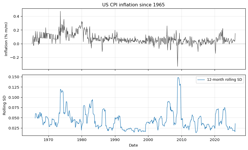
The rolling standard deviation makes the regime shift obvious. Volatility is elevated in the 1970s, spikes around the early-1980s disinflation, and then settles into a much narrower band from the mid-1980s onward. A rolling window is a useful diagnostic but it is a crude estimator: the window is fixed, the weights are flat, and the implied volatility at date \(t\) uses data from \(t - 11\) through \(t\) with no pooling toward a prior or adjacent periods. The SV model will give us a smoother, probabilistically coherent volatility path.
Model
The random-walk stochastic volatility model is a two-equation state-space system. For the observed series \(y_t\), $\(y_t = \mu + u_t, \qquad u_t \sim N\!\left(0,\, \exp(h_t)\right),\)$ and for the latent log-volatility \(h_t\), $\(h_t = h_{t-1} + \sigma_\eta\, \eta_t, \qquad \eta_t \sim N(0, 1).\)$ Here \(\mu\) is the unconditional mean of the series, \(h_t\) is the log of the conditional variance at date \(t\), and \(\sigma_\eta\) controls how fast log-volatility can move from one period to the next. The conditional standard deviation at \(t\) is \(\exp(h_t / 2)\), so a one-unit increase in \(h_t\) multiplies the conditional SD by \(e^{1/2} \approx 1.65\).
Modelling log-volatility rather than the variance or the SD directly has two practical advantages. First, \(\exp(h_t)\) is strictly positive for any real-valued \(h_t\), so the parameterisation cannot wander into infeasible regions. Second, movements in \(h_t\) are symmetric: a change of \(+0.5\) and a change of \(-0.5\) correspond to multiplicative moves of the same magnitude in the SD, which makes the random-walk innovation assumption more plausible.
State-space structure and what it implies
The two equations define a linear Gaussian state-space system in which the latent state controls the observation variance rather than the mean. Conditional on the full path \(h_{1:T}\) the likelihood factorises, $\(p(y_{1:T} \mid h_{1:T}, \mu) \;=\; \prod_{t=1}^{T} N\!\left(y_t;\, \mu,\, \exp(h_t)\right),\)$ and each factor is cheap. The likelihood of the parameters \((\mu, \sigma_\eta)\) alone requires integrating the latent path out, $\(p(y_{1:T} \mid \mu, \sigma_\eta) \;=\; \int p(y_{1:T} \mid h_{1:T}, \mu)\, p(h_{1:T} \mid \sigma_\eta)\, dh_{1:T}.\)$ This \(T\)-dimensional integral has no closed form, which is why SV models are fit with MCMC or particle methods rather than direct maximum likelihood. MCMC sidesteps the integral by sampling the joint posterior \(p(\mu, \sigma_\eta, h_{1:T} \mid y_{1:T})\) and reading off any marginal we need from the draws.
Marginally over \(h_t\), the observation is a scale mixture of normals: \(y_t = \mu + \exp(h_t / 2)\,\varepsilon_t\) with \(\varepsilon_t \sim N(0, 1)\) independent of \(h_t\). Three consequences follow that a fixed-variance model cannot reproduce. The marginal distribution of \(y_t\) has heavier tails than a Gaussian. Squared residuals \((y_t - \mu)^2\) are positively autocorrelated — volatility clustering. And a realised large \(|y_t|\) is evidence of a large \(h_t\), which raises the posterior probability that \(|y_{t+1}|\) is also large. These are exactly the stylised facts that motivate the model for macro and financial series.
It is worth contrasting this setup with the GARCH family, which targets the same stylised facts by a different route. In GARCH, the conditional variance is a deterministic function of past observations, \(h_t = \omega + \alpha\,(y_{t-1} - \mu)^2 + \beta\,h_{t-1}\), so given \((y_{1:t-1}, \omega, \alpha, \beta)\) the variance at \(t\) is a known number and the likelihood factorises without an integral. The SV variance has its own innovation \(\eta_t\) that is not observed, which makes it a random variable even after conditioning on the full history. That extra source of randomness is what lets SV allow volatility surprises — moments when the conditional variance jumps in a way not foreseeable from past squared returns — and it is also the reason the SV likelihood is intractable in closed form.
The random-walk specification for \(h_t\) is non-stationary. Conditional on \(h_0\), $\(h_t \mid h_0, \sigma_\eta \;\sim\; N\!\left(h_0,\, t\,\sigma_\eta^2\right),\)$ so the unconditional variance of log-volatility grows linearly in \(t\). That is the appropriate prior when there is no reason to anchor volatility to a particular level and we want the data to decide how far it drifts. The AR(1) variant introduced later replaces this with a mean-reverting state equation and restores stationarity.
!!! note “NUTS on the SV likelihood”
We sample the SV model with PyMC's NUTS using a non-centered reparameterisation of the latent log-volatility path. Non-centering lets Hamiltonian Monte Carlo traverse the funnel geometry induced by $\sigma_\eta$ without the auxiliary-mixture approximation introduced by Kim, Shephard and Chib (1998) to make the likelihood conditionally Gaussian.
Fitting the random-walk SV model
We wrap the inflation series in an SVData container and fit a StochasticVolatility model with random-walk log-vol dynamics.
data = SVData.from_series(inflation, name="inflation")

if ci:
    sampler = NUTSSampler(draws=10, tune=50, chains=1, cores=1, random_seed=123)
else:
    sampler = NUTSSampler(
        draws=1500,
        tune=3000,
        chains=4,
        cores=4,
        target_accept=0.95,
        random_seed=123,
    )

fitted = StochasticVolatility(dynamics="random_walk").fit(data, sampler=sampler)
Sampler Progress
Total Chains: 4
Active Chains: 0
Finished Chains: 4
Sampling for 27 seconds
Estimated Time to Completion: now
| Progress | Draws | Divergences | Step Size | Gradients/Draw |
|---|---|---|---|---|
| 4500 | 0 | 0.02 | 511 | |
| 4500 | 0 | 0.02 | 511 | |
| 4500 | 0 | 0.02 | 511 | |
| 4500 | 0 | 0.02 | 511 |
The posterior volatility path
fitted.volatility() returns a VolatilityResult whose .plot() method shows the posterior median of \(\exp(h_t / 2)\) together with a highest-density interval.

To see how the volatility path lines up with the macroeconomic narrative we overlay NBER recession dates that fall within the sample. These are the recessions dated by the NBER Business Cycle Dating Committee from 1965 onward.
fig = fitted.volatility().plot()
ax = plt.gcf().axes[0]
nber_recessions = [
    ("1969-12", "1970-11"),
    ("1973-11", "1975-03"),
    ("1980-01", "1980-07"),
    ("1981-07", "1982-11"),
    ("1990-07", "1991-03"),
    ("2001-03", "2001-11"),
    ("2007-12", "2009-06"),
    ("2020-02", "2020-04"),
]
for start, end in nber_recessions:
    ax.axvspan(pd.to_datetime(start), pd.to_datetime(end), alpha=0.15, color="gray")
fig.tight_layout()
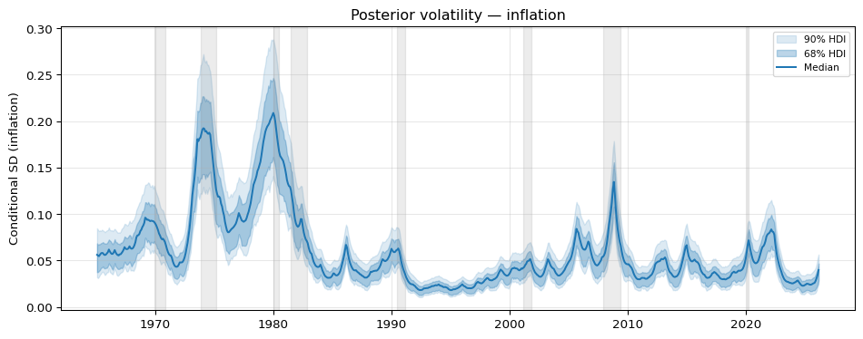
The posterior volatility is elevated throughout the 1970s and peaks during the 1973-75 and 1980-82 recessions. From the mid-1980s onward the conditional SD drops to roughly a third of its 1970s level — the Great Moderation signature that a constant-variance model could not capture — with only mild bumps around the 1990-91 and 2001 recessions. The 2007-09 financial crisis produces a visible uptick, and the 2020 COVID shock and the post-2021 inflation surge push the conditional SD back toward levels not seen since the early 1980s.
Posterior SD versus rolling SD
How does the SV posterior compare with the naive 12-month rolling estimator we plotted earlier? We overlay them on the same axes.
posterior_sd = fitted.volatility().median()

fig, ax = plt.subplots(figsize=(9, 4))
ax.plot(
    rolling_sd.index,
    rolling_sd.values,
    color="0.55",
    linewidth=1.0,
    label=f"{rolling_window}-month rolling SD",
)
ax.plot(
    posterior_sd.index,
    posterior_sd["inflation"].values,
    color="C0",
    linewidth=1.5,
    label="SV posterior median SD",
)
ax.set_ylabel("Conditional SD")
ax.set_xlabel("Date")
ax.legend(loc="upper right", fontsize=9)
ax.grid(alpha=0.3)
ax.set_title("SV posterior SD vs rolling SD — US CPI inflation")
fig.tight_layout()
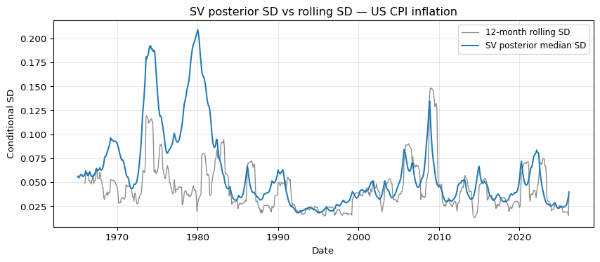
Both estimators agree on the overall shape: high in the 1970s and early 1980s, low from the mid-1980s onward. The SV posterior is visibly smoother and avoids the sharp step changes the rolling estimator produces when a single unusual month enters or leaves the window. The posterior also pools information across the full sample through the random-walk prior on \(h_t\), whereas the rolling SD uses only the most recent 12 observations.
The gap between the two estimators is most striking in the 1970s and early 1980s, and it almost vanishes in 2008 and 2020. That asymmetry is not about volatility at all — it is about how each estimator treats the mean. The rolling SD subtracts a local 12-month average before squaring, so slow drift in the level of inflation is absorbed into the mean and never shows up as variance. The SV model has a single global \(\mu\), so every observation is residualised against one constant over the whole sample. When inflation ran at roughly 1% a month for years at a stretch, those deviations from the full-sample mean were enormous, and \(\exp(h_t/2)\) had to stretch to accommodate them. The spikes in 2008 and 2020 were short and the level around them was close to the long-run mean, so a local window and a global constant see almost the same residuals and the two lines coincide.
AR(1) dynamics for log-volatility
The random-walk specification places no anchor on the level of log-volatility: if \(\sigma_\eta\) is small the path drifts slowly, if it is large the path wanders. An AR(1) alternative adds explicit mean reversion, $\(h_t = \alpha + \phi\,(h_{t-1} - \alpha) + \sigma_\eta\, \eta_t,\)$ with \(|\phi| < 1\). This lets the data speak to whether log-volatility tends to return to a long-run level \(\alpha\) and, if so, how fast. A persistence parameter \(\phi\) posterior concentrated near 1 is consistent with the random-walk approximation being adequate; values meaningfully below 1 indicate stronger mean reversion than a pure random walk allows.
Instead of the "ar1" shorthand used above, we pass an explicit AR1() dynamics object. Both forms are equivalent; the object form is the extension point if you want to add a new dynamics (e.g. SVt or SV with leverage) without editing the library — implement the SVDynamics protocol and pass an instance here.
if ci:
    sampler_ar1 = NUTSSampler(draws=10, tune=50, chains=1, cores=1, random_seed=321)
else:
    sampler_ar1 = NUTSSampler(
        draws=1500,
        tune=3000,
        chains=4,
        cores=4,
        target_accept=0.95,
        random_seed=321,
    )

fitted_ar1 = StochasticVolatility(dynamics=AR1()).fit(data, sampler=sampler_ar1)
fig_ar1 = fitted_ar1.volatility().plot()
fig_ar1.tight_layout()
Sampler Progress
Total Chains: 4
Active Chains: 0
Finished Chains: 4
Sampling for now
Estimated Time to Completion: now
| Progress | Draws | Divergences | Step Size | Gradients/Draw |
|---|---|---|---|---|
| 4500 | 0 | 0.09 | 127 | |
| 4500 | 0 | 0.09 | 127 | |
| 4500 | 0 | 0.08 | 127 | |
| 4500 | 0 | 0.09 | 127 |
The AR(1) volatility path should look qualitatively similar to the random-walk version on the bulk of the sample. The two disagree mostly at the tails, where the AR(1) prior pulls the path toward \(\alpha\) while the random walk lets it drift. Inspecting the posterior of \(\phi\) is the quickest way to decide whether that mean reversion is informative: if the mass sits very close to 1, the two specifications are almost indistinguishable.
Density forecasts
With the random-walk SV fit we can generate a density forecast. For each posterior draw we simulate forward 12 months by evolving \(h_{T+h}\) as \(h_T + \sum_{s=1}^{h} \sigma_\eta \eta_s\) and then drawing \(y_{T+h} = \mu + \exp(h_{T+h}/2)\, \varepsilon_{T+h}\).
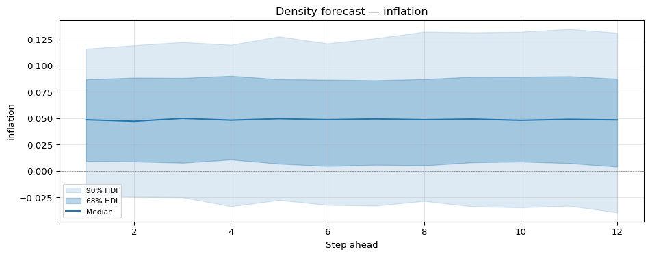
In principle the fan should widen with horizon: \(\mathrm{Var}(h_{T+h}\mid h_T,\sigma_\eta) = h\,\sigma_\eta^2\) grows linearly in \(h\), and \(\mathrm{Var}(y_{T+h})\) inherits an \(\exp(0.5\, h\, \sigma_\eta^2)\) factor on top of \(\exp(h_T)\). In practice the visible widening here is modest: the posterior \(\sigma_\eta\) for monthly CPI inflation is small, so over twelve steps the forward-dispersion factor on the conditional SD is only a few percent, and the bulk of the fan width comes from posterior uncertainty in \(h_T\) itself rather than from forward dispersion. Pushing the horizon out further, or using a series with a larger \(\sigma_\eta\), makes the geometric growth easier to see.
Stochastic volatility inside a VAR
The same monetary_policy.csv we loaded earlier already carries a multivariate macro panel (output, prices, rate). To swap the homoscedastic VAR for one with multivariate Clark-style stochastic volatility, pass volatility="sv" (or a StochasticVolatility(...) instance) when constructing the spec:
from impulso import VAR, VARData
from impulso.identification import Cholesky

var_data = VARData.from_df(df, endog=["output", "prices", "rate"])

if ci:
    sampler_var = NUTSSampler(draws=10, tune=50, chains=1, cores=1, random_seed=7)
else:
    sampler_var = NUTSSampler(
        draws=500,
        tune=1000,
        chains=2,
        cores=1,  # cores=1 avoids the macOS multiprocessing segfault
        target_accept=0.95,
        random_seed=7,
    )

fitted_var = VAR(lags=2, volatility="sv").fit(var_data, sampler=sampler_var)
Sampler Progress
Total Chains: 2
Active Chains: 0
Finished Chains: 2
Sampling for 5 minutes
Estimated Time to Completion: now
| Progress | Draws | Divergences | Step Size | Gradients/Draw |
|---|---|---|---|---|
| 1500 | 241 | 0.01 | 457 | |
| 1500 | 183 | 0.01 | 174 |
For a constant-volatility VAR, FittedVAR.sigma() returns a single covariance matrix per posterior draw, shape (chains, draws, n_vars, n_vars). With volatility="sv" it returns a full per-period path:
(2, 500, 732, 3, 3)
The per-variable log-volatility paths live in the posterior under the stacked h deterministic, shape (chains, draws, T_eff, n_vars):
('chain', 'draw', 'h_dim_0', 'h_dim_1') (2, 500, 732, 3)
Time-varying impulse responses with at=
When the volatility is time-varying, the structural impact matrix is too. The at= parameter on impulse_response, fevd, and historical_decomposition selects which date’s Cholesky factor (and hence which structural impact matrix) the computation uses:
at="last"— most recent in-sample period (the default when the volatility is stochastic)at=t— a specific integer index into the lag-trimmed sampleat="all"— every in-sample period; the result carries atimedim
For constant-volatility VARs, at= is a no-op (the same L applies at every date), so existing tutorials that omit it keep working unchanged.
identified = fitted_var.set_identification_strategy(
    Cholesky(ordering=["output", "prices", "rate"])
)
A single date — the most recent in-sample period:
irf_latest = identified.impulse_response(horizon=12, at="last")
irf_latest_arr = irf_latest.idata.posterior_predictive["irf"]
print(irf_latest_arr.shape)  # (chains, draws, horizon+1, n_vars, n_vars)
(2, 500, 13, 3, 3)
A specific historical date. The integer index is into the lag-trimmed sample, so we offset by n_lags when resolving from the calendar index:
trimmed_index = var_data.index[fitted_var.n_lags :]
t_1982 = trimmed_index.get_loc("1982-01-01")
irf_1982 = identified.impulse_response(horizon=12, at=t_1982)
print(irf_1982.idata.posterior_predictive["irf"].shape)
(2, 500, 13, 3, 3)
Every in-sample date in one call. The result is a six-dimensional array — (chains, draws, time, horizon+1, n_vars, n_vars) — that you usually post-process directly via irf_all.idata rather than .median() / .plot(), which intentionally raise for the time-aware result:
irf_all = identified.impulse_response(horizon=12, at="all")
irf_all_arr = irf_all.idata.posterior_predictive["irf"]
print(irf_all_arr.shape)
print(irf_all_arr.dims)
(2, 500, 732, 13, 3, 3)
('chain', 'draw', 'time', 'horizon', 'response', 'shock')
The same at= argument is accepted by fevd and historical_decomposition with the same semantics.
References
- Carriero, A., Clark, T. E., and Marcellino, M. (2016). Common drifting volatility in large Bayesian VARs. Journal of Applied Econometrics, 31(2), 375-404.
- Clark, T. E. (2011). Real-time density forecasts from Bayesian vector autoregressions with stochastic volatility. Journal of Business and Economic Statistics, 29(3), 327-341.
- Cogley, T., and Sargent, T. J. (2005). Drifts and volatilities: Monetary policies and outcomes in the post-WWII U.S. Review of Economic Dynamics, 8(2), 262-302.
- Kim, S., Shephard, N., and Chib, S. (1998). Stochastic volatility: Likelihood inference and comparison with ARCH models. Review of Economic Studies, 65(3), 361-393.
- Primiceri, G. E. (2005). Time varying structural vector autoregressions and monetary policy. Review of Economic Studies, 72(3), 821-852.