The conjugate VAR: fast Bayesian estimation

When to reach for ConjugateVAR instead of the NUTS VAR

Impulso estimates a reduced-form VAR two ways. Both return the same FittedVAR, so identification, impulse responses, FEVDs, and forecasts are byte-for-byte identical downstream. What differs is the mode of inference:

• The NUTS VAR (VAR) places independent-Normal priors on the coefficients and samples the full posterior with Hamiltonian Monte Carlo. Maximally flexible — it admits per-equation shrinkage, stochastic volatility, sign restrictions, and external instruments — but every coefficient is a sampled latent, so large systems are slow.

• The conjugate VAR (ConjugateVAR) places a Normal-Inverse-Wishart prior, which is conjugate to the VAR likelihood. The coefficient/covariance posterior is then available in closed form: we draw \((\beta, \Sigma)\) analytically and reserve Monte Carlo for a single low-dimensional hyperparameter — the Minnesota tightness \(\lambda\) — which the data selects by marginal likelihood (Giannone et al. [2015]).

This notebook fits both on the same series, shows they reach the same structural conclusions, times them, and ends with a rule for choosing between them. We use an environmental system — a German climate–energy VAR — rather than the usual macro data, to show the machinery is domain-agnostic.

Scope

This is the estimator-first tour. For the conjugate VAR wearing a deterministic volatility break — the COVID application it was built for — see Estimating a VAR after March 2020. Why a conjugate estimator is a sibling of VAR rather than a mode of it is recorded in ADR 0004.

import time

import arviz as az
import matplotlib.pyplot as plt
import numpy as np
import pandas as pd
from qc_core import plotting

from impulso import Cholesky, ConjugateVAR, MinnesotaPrior, NIWPrior, VAR, VARData, compare_evidence
from impulso.samplers import NUTSSampler

plotting.use_ledger_style()

Data: a German climate–energy system

Weather is where the environment meets the economy: temperature drives heating and cooling demand, sunshine and wind set renewable supply, and rainfall feeds hydro and agriculture. We assemble a four-variable monthly system for Berlin (1980–2024) from the ERA5 reanalysis (Hersbach and others [2020]), served by the Open-Meteo historical archive.

Variable	ERA5 series (monthly mean of daily)	Unit	Economic reading
temperature	temperature_2m_mean	°C	heating / cooling demand
radiation	shortwave_radiation_sum	MJ/m²	solar-PV potential
wind	wind_speed_10m_mean	km/h	wind-power potential
precipitation	precipitation_sum	mm/day	hydro / runoff

The committed CSV is produced once by scripts/fetch_berlin_climate.py and read offline here — no network call at render time. That script targets Open-Meteo’s free archive endpoint, so anyone can reproduce the file without credentials.

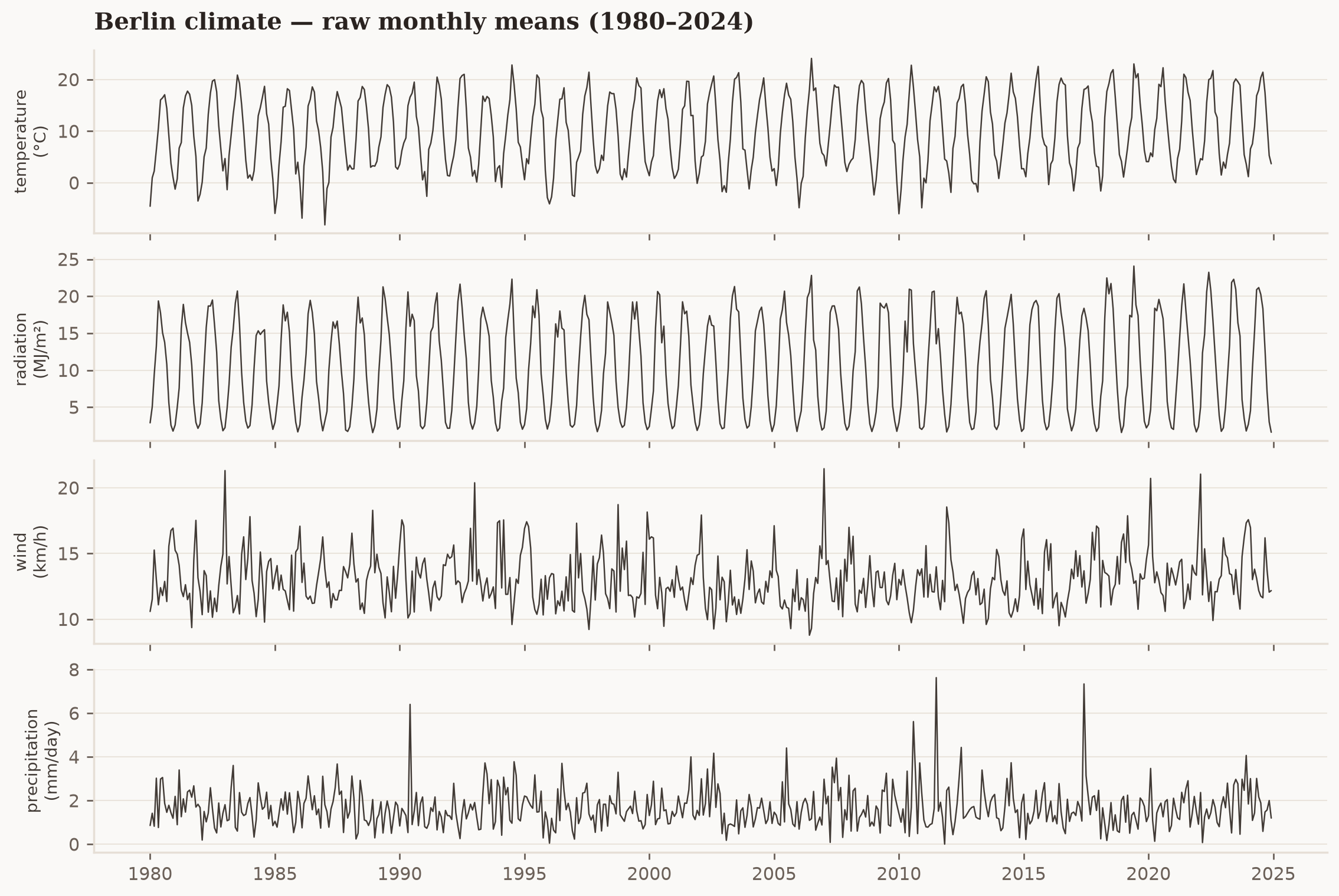
Fig. 15 Raw monthly ERA5 series for Berlin, 1980–2024. Temperature and radiation are dominated by the seasonal cycle.

The raw series are overwhelmingly seasonal — a VAR fit on them would spend its coefficients re-learning the calendar. We model anomalies instead: each observation minus its month-of-year climatological mean, standardised to unit variance. The result is stationary, comparable across variables, and lets impulse responses read in standard deviations.

climatology = raw.groupby(raw.index.month).transform("mean")
anomalies = raw - climatology
anomalies = (anomalies - anomalies.mean()) / anomalies.std()
anomalies.describe().round(2)

	temperature	radiation	wind	precipitation
count	540.00	540.00	540.00	540.00
mean	0.00	0.00	-0.00	0.00
std	1.00	1.00	1.00	1.00
min	-4.30	-4.51	-2.74	-2.10
25%	-0.58	-0.45	-0.69	-0.67
50%	0.00	-0.01	-0.05	-0.13
75%	0.63	0.43	0.56	0.54
max	2.79	3.72	4.02	6.04

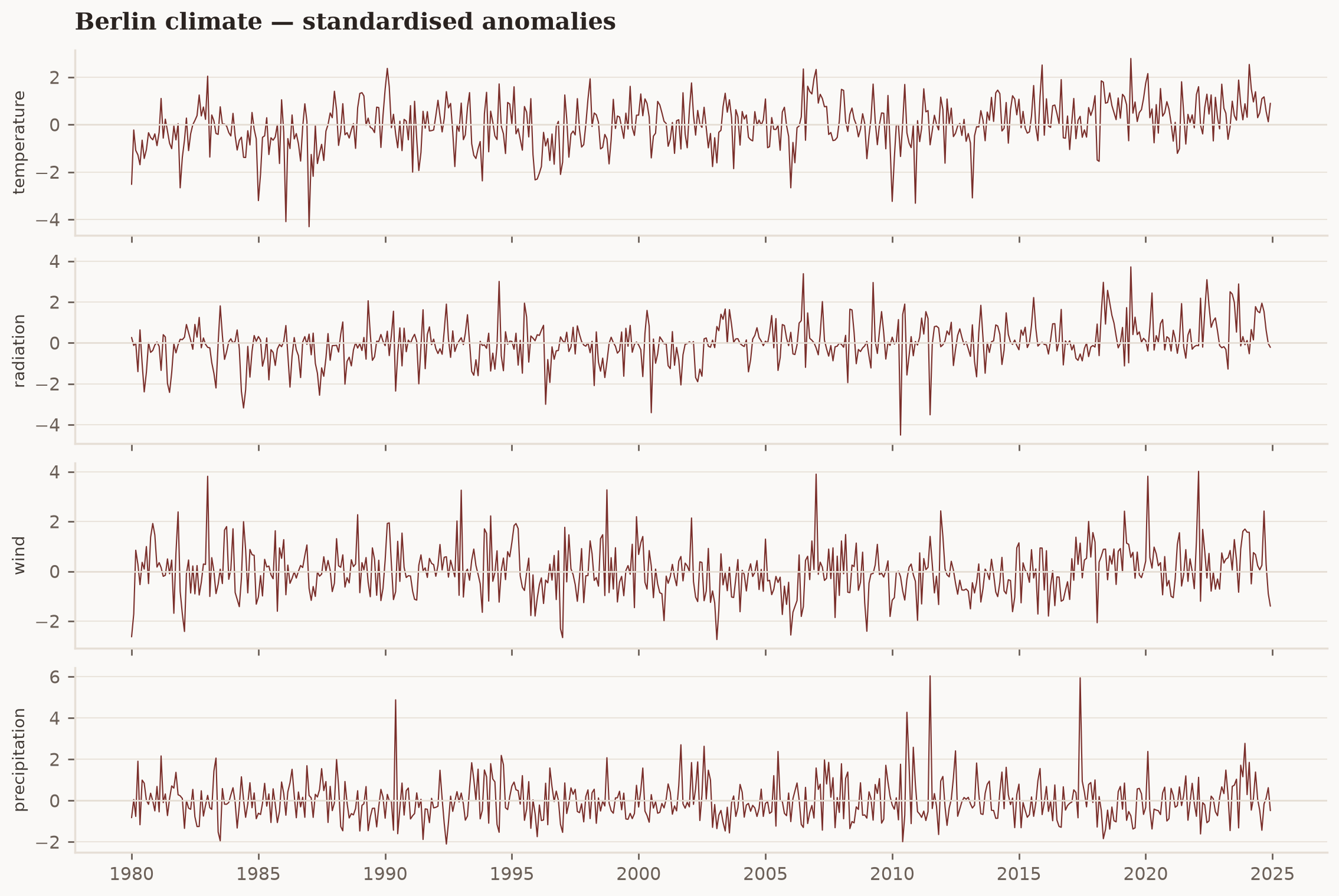
Fig. 16 Standardised monthly anomalies — the seasonal cycle removed. This is what the VAR sees.

Fitting the conjugate VAR

We use twelve lags — enough to capture up to a year of dynamic feedback in monthly data — giving \(4 \times 12 = 48\) coefficients per equation. The prior is the conjugate Minnesota prior NIWPrior; select=True asks the estimator to choose the overall tightness \(\lambda\) by maximising the marginal likelihood and then sample its posterior, rather than fixing it by hand (Giannone et al. [2015]; the Minnesota shrinkage idea goes back to Doan et al. [1984] and Litterman [1986]).

LAGS = 12
data = VARData.from_df(anomalies, endog=list(anomalies.columns))

conjugate_prior = NIWPrior(select=True, decay=2.0, cross_shrinkage=1.0)
start = time.perf_counter()
fitted_conjugate = ConjugateVAR(lags=LAGS, prior=conjugate_prior, draws=2000, tune=1000, seed=0).fit(data)
conjugate_seconds = time.perf_counter() - start

lambda_hat = float(fitted_conjugate.idata.posterior["lambda_"].median())
print(f"data-selected Minnesota tightness  lambda = {lambda_hat:.3f}")
print(f"conjugate fit wall-clock                  = {conjugate_seconds:.2f} s")

data-selected Minnesota tightness  lambda = 0.271
conjugate fit wall-clock                  = 3.10 s

The estimator reports a posterior for \(\lambda\) (not a fixed value): the data speak to how much shrinkage the system needs. Everything downstream — coefficients, covariance, the base Cholesky factor — was drawn in closed form conditional on those hyperparameter draws.

The same model by NUTS

To make this a clean inference-mode comparison, we fit the NUTS VAR at the same tightness the conjugate estimator just selected (MinnesotaPrior(tightness=lambda_hat)). Now the only differences are the prior family (independent-Normal vs conjugate NIW) and the sampler — not the amount of shrinkage.

if ci:
    sampler = NUTSSampler(
        draws=50,
        tune=500,
        chains=1,
        cores=1,
        target_accept=0.9,
        random_seed=0,
        nuts_sampler_kwargs={"low_rank_modified_mass_matrix": True},
    )
else:
    sampler = NUTSSampler(draws=1000, tune=1500, chains=2, cores=1, random_seed=0)

start = time.perf_counter()
fitted_nuts = VAR(lags=LAGS, prior=MinnesotaPrior(tightness=lambda_hat)).fit(data, sampler=sampler)
nuts_seconds = time.perf_counter() - start
print(f"NUTS fit wall-clock = {nuts_seconds:.2f} s")
az.summary(fitted_nuts.idata, var_names=["intercept"], kind="diagnostics")

NUTS fit wall-clock = 71.38 s

	mcse_mean	mcse_sd	ess_bulk	ess_tail	r_hat
intercept[temperature]	0.001	0.001	3916.0	1763.0	1.01
intercept[radiation]	0.001	0.001	3430.0	1530.0	1.00
intercept[wind]	0.001	0.001	3190.0	1759.0	1.00
intercept[precipitation]	0.001	0.001	3421.0	1689.0	1.00

Speed

Both estimators fit the identical 4-variable, 12-lag system. The conjugate path spends Monte Carlo only on a single scalar; NUTS explores a ~200-dimensional coefficient posterior. At full render the gap is an order of magnitude or more.

if ci:
    print("CI smoke mode: NUTS is shrunk to a few draws — these timings are NOT representative.")
else:
    print(
        f"conjugate: {conjugate_seconds:.2f} s | "
        f"NUTS: {nuts_seconds:.2f} s | "
        f"speed-up: {nuts_seconds / conjugate_seconds:.0f}x"
    )

conjugate: 3.10 s | NUTS: 71.38 s | speed-up: 23x

Downstream parity: identical structural machinery

Because both estimators return a FittedVAR, identification is the same call on each. We apply a Cholesky scheme with the ordering radiation → temperature → wind → precipitation (solar forcing is the most exogenous; rainfall the most responsive). The ordering encodes real assumptions — see Monetary Policy Analysis for how much it can matter — but here we hold it fixed and vary only the estimator.

ordering = ["radiation", "temperature", "wind", "precipitation"]
irf_conjugate = fitted_conjugate.set_identification_strategy(Cholesky(ordering=ordering)).impulse_response(horizon=24)
irf_nuts = fitted_nuts.set_identification_strategy(Cholesky(ordering=ordering)).impulse_response(horizon=24)

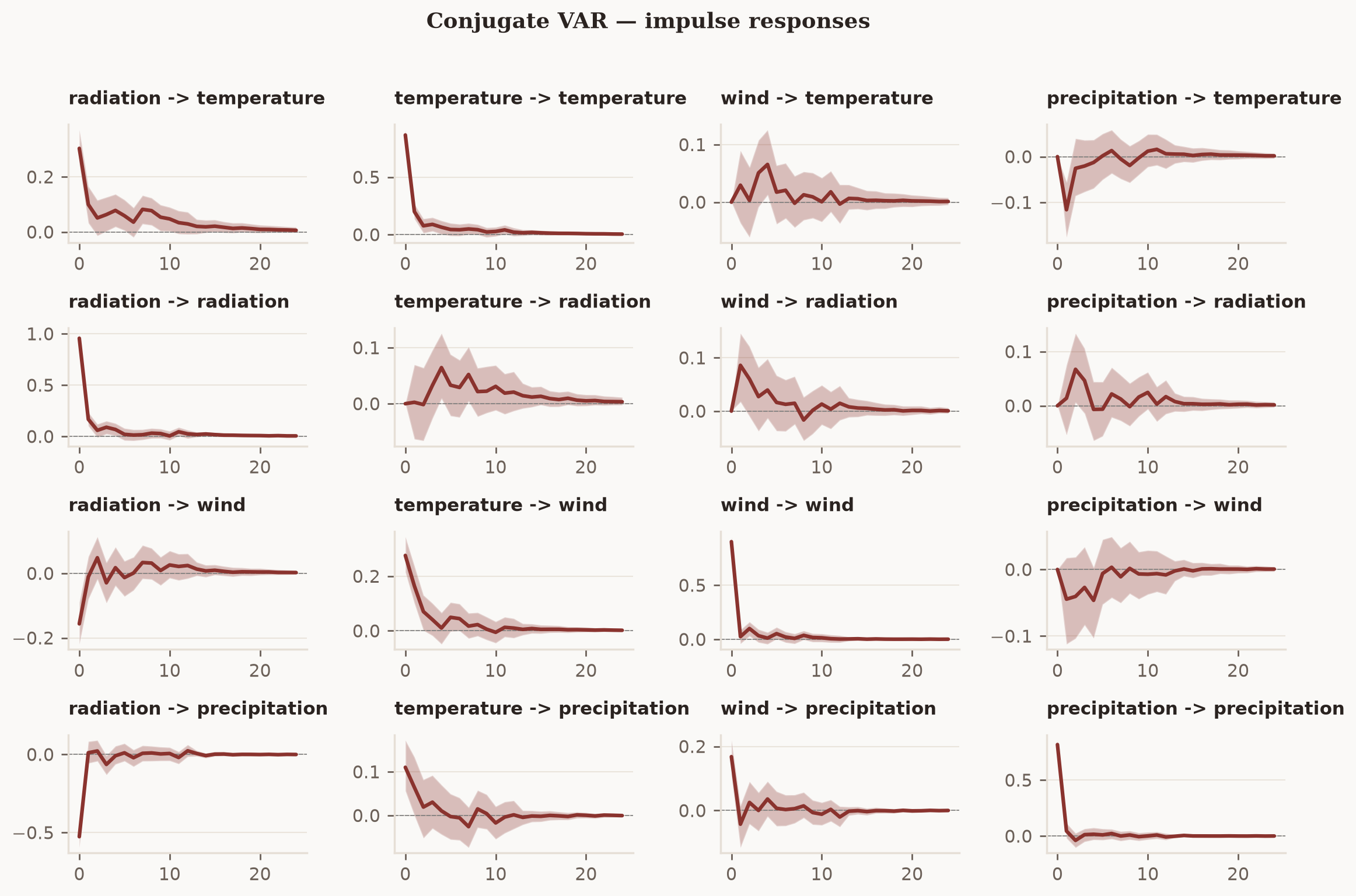
Fig. 17 Conjugate-VAR impulse responses (Cholesky). Column shock → row response, over 24 months.

Now overlay the two estimators on the same axes. If the conjugate VAR is a legitimate estimator and not a shortcut, its responses should track the NUTS responses in shape and sign, with band widths of the same order.

def irf_band(irf_result, shock, response, prob=0.9):
    """Return (horizons, median, hdi_low, hdi_high) for one shock→response pair."""
    draws = irf_result.idata.posterior_predictive["irf"].sel(shock=shock, response=response)
    median = draws.median(dim=("chain", "draw")).values
    hdi = az.hdi(draws, hdi_prob=prob)["irf"]
    return np.arange(median.shape[0]), median, hdi.sel(hdi="lower").values, hdi.sel(hdi="higher").values

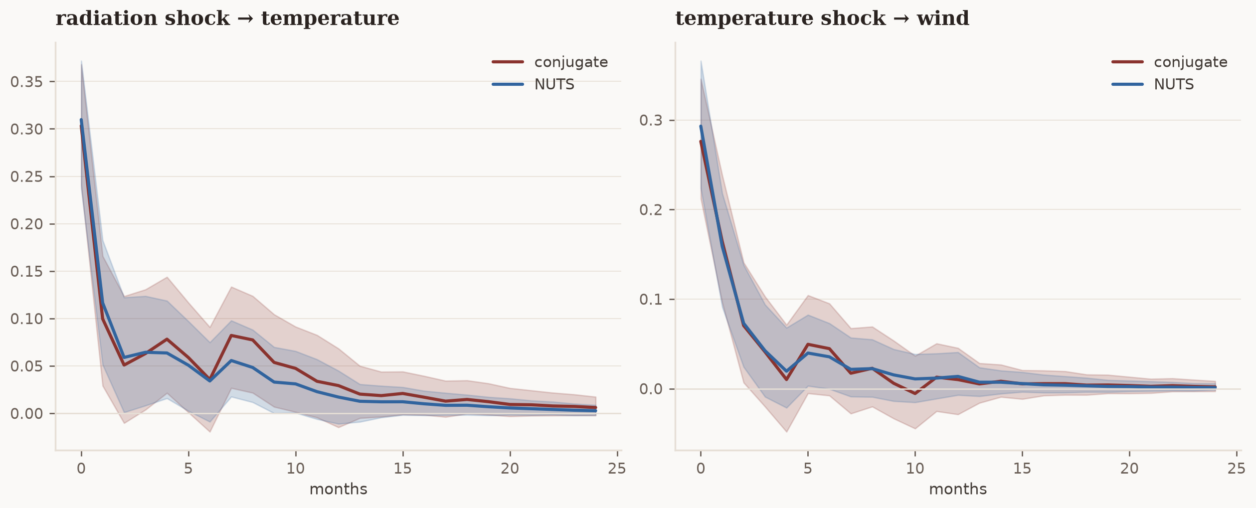
Fig. 18 Conjugate vs NUTS impulse responses at the same tightness. Medians (lines) and 90% bands (shaded).

The two estimators tell the same structural story: a positive radiation (sunshine) shock warms temperature; a warmth shock is followed by calmer winds. The medians track closely and the bands overlap. They are not identical — the conjugate NIW prior imposes a symmetric Kronecker structure across equations while the NUTS prior is independent-Normal — and that is exactly the point: the inference mode is a modelling choice, not a source of contradiction.

if not ci:
    correlations = [
        np.corrcoef(irf_band(irf_conjugate, shock, response)[1], irf_band(irf_nuts, shock, response)[1])[0, 1]
        for shock in ordering
        for response in ordering
    ]
    print(f"median-IRF shape correlation across all 16 shock/response pairs: {np.nanmean(correlations):.2f}")

median-IRF shape correlation across all 16 shock/response pairs: 0.98

Which lag order does the data prefer?

The closed form gives us more than speed. Every conjugate fit reports its marginal likelihood — the density of the observed data under the model, with the coefficients and covariance integrated out — on fitted.evidence. Ratios of those numbers are Bayes factors, so the twelve-lag choice we made by convention can be put to the data instead.

One alignment matters. A VAR(\(p\)) conditions on its first \(p\) rows and models the rest, so a VAR(1) and a VAR(12) on the same DataFrame are densities over different observations and their ratio means nothing. We therefore feed each candidate a series pre-trimmed to the longest lag order, anomalies.iloc[LAGS - p:], so all three model exactly the same response window and differ only in how far back they look. compare_evidence refuses the comparison — loudly — if that alignment is missing.

comparison_draws = 50 if ci else 250
candidates = {}
for p in (1, 6, LAGS):
    aligned = VARData.from_df(anomalies.iloc[LAGS - p :], endog=list(anomalies.columns))
    candidates[f"p{p}"] = ConjugateVAR(
        lags=p,
        prior=NIWPrior(select=True, decay=2.0, cross_shrinkage=1.0),
        draws=comparison_draws,
        tune=comparison_draws,
        seed=0,
    ).fit(aligned)

evidence = compare_evidence(**candidates)
print(f"preferred lag order: {evidence.best}")
evidence.to_dataframe().round(3)

preferred lag order: p1

	log_marginal_likelihood	log_bayes_factor	log10_bayes_factor	bayes_factor	posterior_probability	n_obs	n_vars	n_lags	volatility
model
p1	-2887.067	0.000	0.000	1.0	1.0	528	4	1	None
p6	-2915.205	-28.138	-12.220	0.0	0.0	528	4	6	None
p12	-2917.275	-30.208	-13.119	0.0	0.0	528	4	12	None

The log_bayes_factor column reads against the first model passed (p1 here); the log10 column is the unit Kass and Raftery tabulate, and posterior_probability converts the evidences to model weights under a flat prior over the three candidates. On these de-seasonalised anomalies the short model wins by tens of log points: once the calendar is removed, a month of Berlin weather carries little information about the next year of it, and the extra lags buy less than they cost. We keep twelve lags for the rest of the notebook so the estimator comparison stays on the system introduced above — but this is the number to quote when someone asks why.

Two caveats travel with these values. Each is conditional on the presample the shared window leaves in front of it, and each is evaluated at the \(\lambda\) its own fit selected, which makes the ratio an empirical-Bayes Bayes factor rather than a fully marginal one. Both are stated on ModelEvidence.

When to reach for which

Both estimators share the entire post-fitting pipeline — identification, IRFs, FEVDs, forecasts — so the choice is purely about the estimation path.

Reach for the conjugate VAR when…	Reach for the NUTS VAR when…
speed matters — hyperparameter selection, model comparison, or many refits	you need per-equation or asymmetric cross-variable shrinkage
you want the tightness \(\lambda\) chosen by the data (hierarchical)	you need stochastic volatility, sign restrictions, or external instruments
the conjugate NIW (symmetric, Kronecker) prior suits the problem	you need arbitrary or non-conjugate priors
the system is large and full MCMC over every coefficient is costly	you want full HMC convergence diagnostics on all coefficients

The conjugate VAR trades flexibility for closed-form speed and a data-driven prior. When your problem fits inside that trade — as macro and climate systems with symmetric Minnesota shrinkage usually do — it is the sharper tool. When you need volatility that moves or priors that bend per equation, the NUTS VAR is there, and everything you build on top is the same.

We currently have some availability for consulting on how Bayesian modelling, vector autoregressions, and impulso can be integrated into your team's macroeconomic, financial, and environmental forecasting work. If this sounds relevant, book an introductory call. These calls are for consulting inquiries only. For technical usage questions and free community support, please use GitHub Discussions and the documentation.

References

The works cited above are collected on the project bibliography page.