Estimating a VAR after March 2020

In March, April, and May 2020 the U.S. economy moved by amounts that no post-war month had ever recorded. Unemployment jumped from 3.5% in February to 14.7% in April; real consumption collapsed and then rebounded within a quarter. For a linear vector autoregression these three months are not a new regime — they are outliers. A VAR estimates one residual covariance matrix \(\Sigma\) for the whole sample. Three observations that are twenty standard deviations from anything before them inflate that single \(\Sigma\) enormously, and every forecast, impulse response, and credible band inherits the blow-up. Dropping the months is not innocent either: it throws away the most informative episode on record for how consumption responds to a labour-market shock.

Lenza and Primiceri [2022] propose a middle path. Keep every observation, but let the residual volatility rise for the pandemic months and decay smoothly back to normal. Concretely, the residual covariance in month \(t\) becomes \(s_t^2\,\Sigma\), with a common scalar \(s_t\) that equals one before March 2020, takes free values \(\bar s_{\text{Mar}}, \bar s_{\text{Apr}}, \bar s_{\text{May}}\) during the outbreak, and then decays geometrically, \(s_t = 1 + (\bar s_{\text{May}}-1)\,\rho^{\,t-t^\ast-2}\). The change is deliberately minimal: a single common scale multiplies the whole covariance, so the shape of the shock correlations — and therefore the economics of the impulse responses — is preserved, while the size of the shocks is allowed to spike and settle.

This tutorial reproduces that method with Impulso’s conjugate estimator, ConjugateVAR. The scales \(\bar s\) and the decay \(\rho\) are estimated jointly with the prior tightness \(\lambda\) by maximising the closed-form marginal likelihood and sampling around the mode — the hierarchical, empirical-Bayes treatment of \(\lambda\) in Lenza and Primiceri [2022], which is why Figure 1 below includes a posterior for \(\lambda\) alongside the volatility scales.

What this reproduction does and does not match

The paper’s economic design is reproduced faithfully: a seven-variable monthly VAR (unemployment, employment, and five real-consumption / price series), 13 lags, the common-volatility break, and the joint estimation of \(\lambda\) with the outbreak scales. Two boundaries are worth stating plainly.

• Data vintage. The series ship with the docs as a current FRED download, not the real-time 2020 vintage the authors used. Revisions to the 2020 national-accounts data move the numbers slightly, so the posterior scales here will not equal the paper’s to the decimal.

• The conditioning path. The conditional forecast below pins unemployment to a reconstructed trajectory, not the paper’s proprietary Blue Chip consensus path. The early portion mimics the mid-2020 consensus (a slow recovery); the post-2021 portion is a smooth extrapolation, labelled as such, not a survey forecast.

import matplotlib.pyplot as plt
import numpy as np
import pandas as pd

from _post_march_2020 import conditional_forecast
from impulso import Cholesky, ConjugateVAR, NIWPrior, PandemicBreak, VARData

The data and the model panel

The seven series come from FRED (UNRATE, PAYEMS, PCE, PCES, PCEPI, DSERRG3M086SBEA, PCEPILFE), monthly from December 1988 to May 2020. The CSV ships with the documentation, so this notebook makes no network calls at build time. We follow the paper’s transformations: unemployment enters as a level (a rate in percentage points), and every other series enters as \(100\times\log\) of a real quantity — nominal consumption is deflated by its own price index, and the price indices themselves enter in logs. Unemployment is ordered first, which matters later for the Cholesky identification.

raw = pd.read_csv("data/post_march_2020.csv", index_col="date", parse_dates=True)

model_df = pd.DataFrame(index=raw.index)
model_df["unemployment"] = raw["unemployment"]
model_df["employment"] = 100 * np.log(raw["employment"])
model_df["pce"] = 100 * np.log(raw["pce"] / raw["pce_price"])
model_df["pce_services"] = 100 * np.log(raw["pce_services"] / raw["pce_services_price"])
model_df["pce_price"] = 100 * np.log(raw["pce_price"])
model_df["pce_services_price"] = 100 * np.log(raw["pce_services_price"])
model_df["core_pce_price"] = 100 * np.log(raw["core_pce_price"])

assert np.isfinite(model_df.to_numpy()).all(), "model panel contains non-finite values"
var_names = list(model_df.columns)

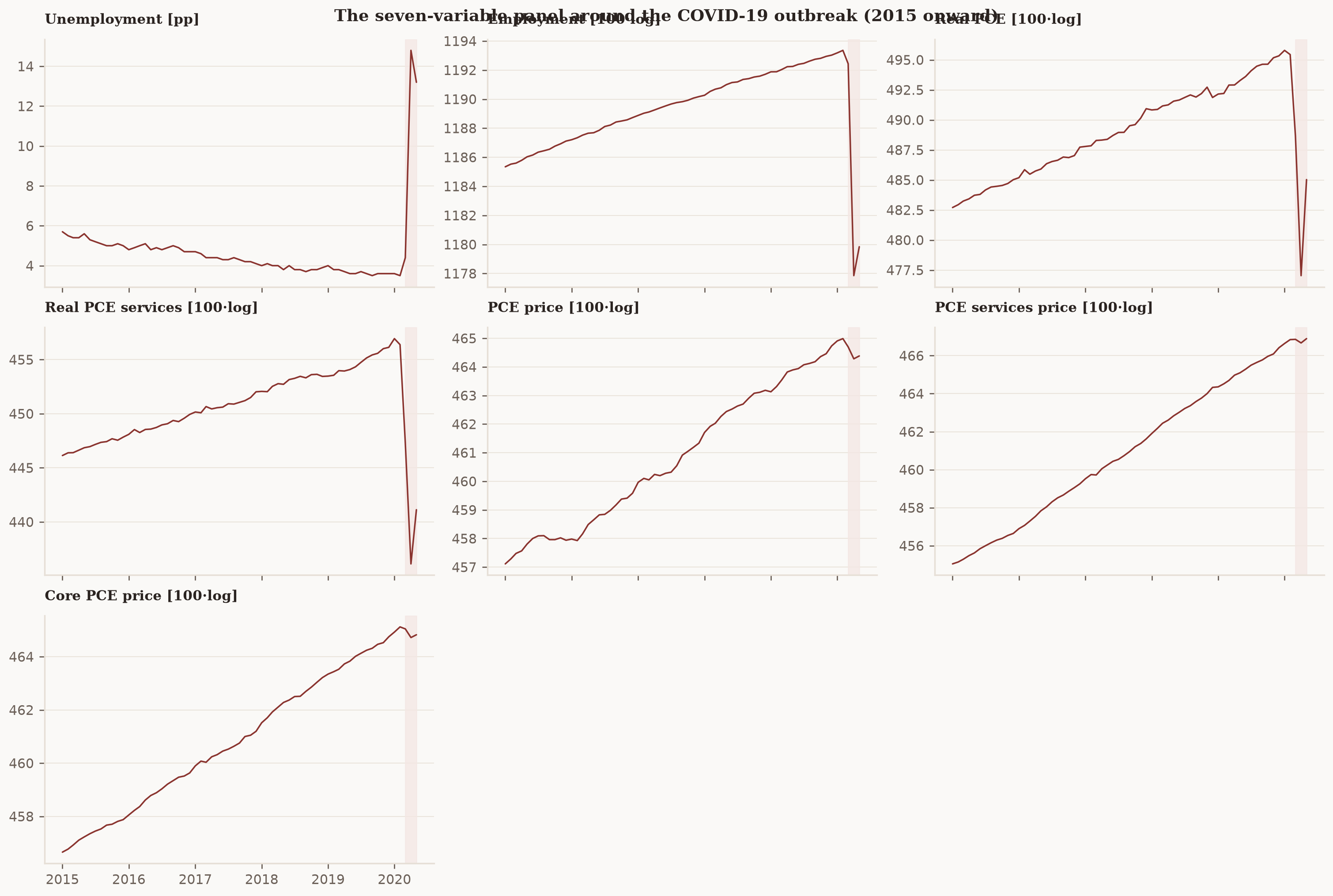
The next figure shows the panel around the pandemic. The March–May 2020 window is shaded. The point of the whole exercise is visible at a glance: three observations lie far outside the range of everything that came before.

Fitting the pandemic VAR

We fit a 13-lag conjugate VAR with the common-volatility break. start is the position of March 2020 (the break date \(t^\ast\)) in the lag-trimmed sample. The prior is NIWPrior(select=True): a natural-conjugate Minnesota prior whose tightness \(\lambda\) is estimated rather than fixed. PandemicBreak adds the three outbreak scales and the decay \(\rho\); all four hyperparameters, together with \(\lambda\), are sampled by random-walk Metropolis around the marginal-likelihood mode.

start = model_df.index[13:].get_loc(pd.Timestamp("2020-03-01"))

fitted = ConjugateVAR(
    lags=13,
    prior=NIWPrior(select=True),
    volatility=PandemicBreak(start=start),
    draws=200 if ci else 2000,
    tune=200 if ci else 2000,
    seed=0,
).fit(VARData.from_df(model_df, endog=var_names))

Figure 1 — the estimated volatility break

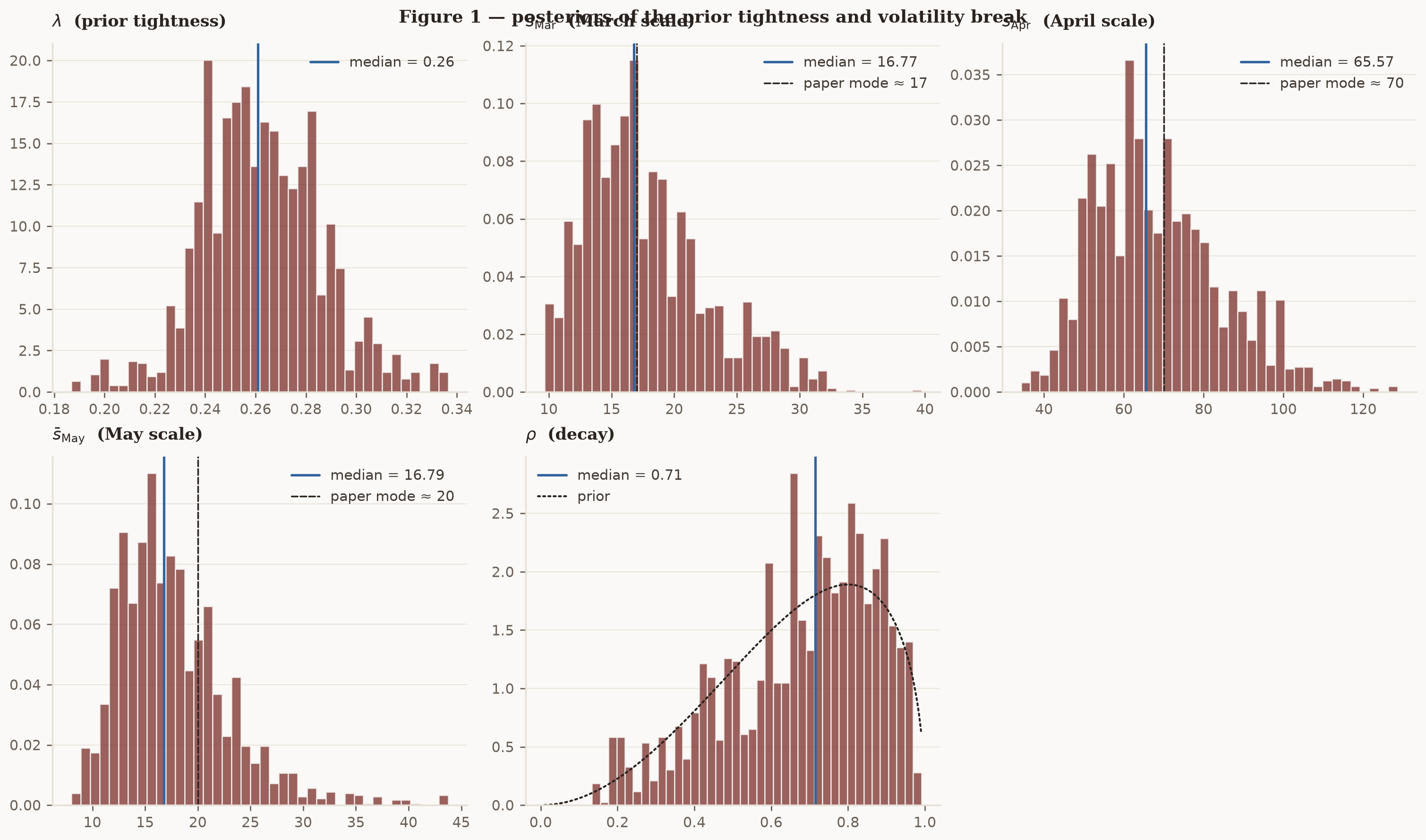
The posteriors below reproduce Figure 1 of the paper. The three outbreak scales are large: the residual standard deviation in March, April, and May 2020 is a double-digit multiple of its normal value, which is exactly why a constant-\(\Sigma\) VAR is distorted by these months. Dashed reference lines mark the scale modes reported in the paper (≈17, ≈70, ≈20). The decay \(\rho\) is shown with its Beta prior overlaid: three months of extreme data pin the scales tightly but say little about the speed of the return to normal, so the \(\rho\) posterior barely moves away from its prior.

The drop-the-pandemic-data baseline

The natural comparison is a VAR that never sees the pandemic. We refit the same specification — same variables, same 13 lags, same conjugate prior — but stop the sample at February 2020 and set volatility=None, so there is no break to estimate. This is the “throw the months away” strategy, and it is the honest alternative the paper argues against.

base_df = model_df.loc[:"2020-02-01"]

fitted_base = ConjugateVAR(
    lags=13,
    prior=NIWPrior(select=True),
    volatility=None,
    draws=200 if ci else 2000,
    tune=200 if ci else 2000,
    seed=0,
).fit(VARData.from_df(base_df, endog=var_names))

Impulse responses: a summary statistic, not a structural shock

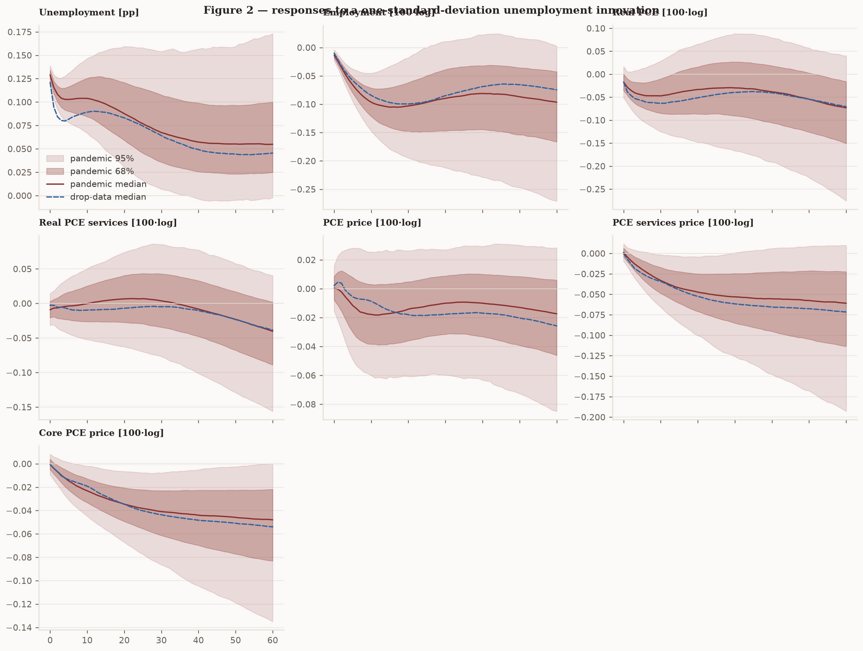
We identify both models with a Cholesky decomposition ordered as the columns appear, unemployment first. For the pandemic model we read the impact matrix at February 2020 — before the break, where the scale is one — so the response is expressed in normal-time units rather than pandemic-inflated ones. The baseline uses its single (constant) covariance.

Read these as descriptive, not causal

A recursive ordering does not deliver a structurally interpretable “unemployment shock” in this system. The lower-triangular factor is a convenient basis for summarising co-movement, and that is all we claim here: the responses describe how the variables typically move together following a one-standard-deviation innovation to unemployment, following the paper’s own caveat against over-interpreting the recursive shock.

chol = Cholesky(ordering=var_names)
irf_at = model_df.index[13:].get_loc(pd.Timestamp("2020-02-01"))

irf_pandemic = fitted.set_identification_strategy(chol).impulse_response(horizon=60, at=irf_at)
irf_baseline = fitted_base.set_identification_strategy(chol).impulse_response(horizon=60)

A conditional forecast for the recovery

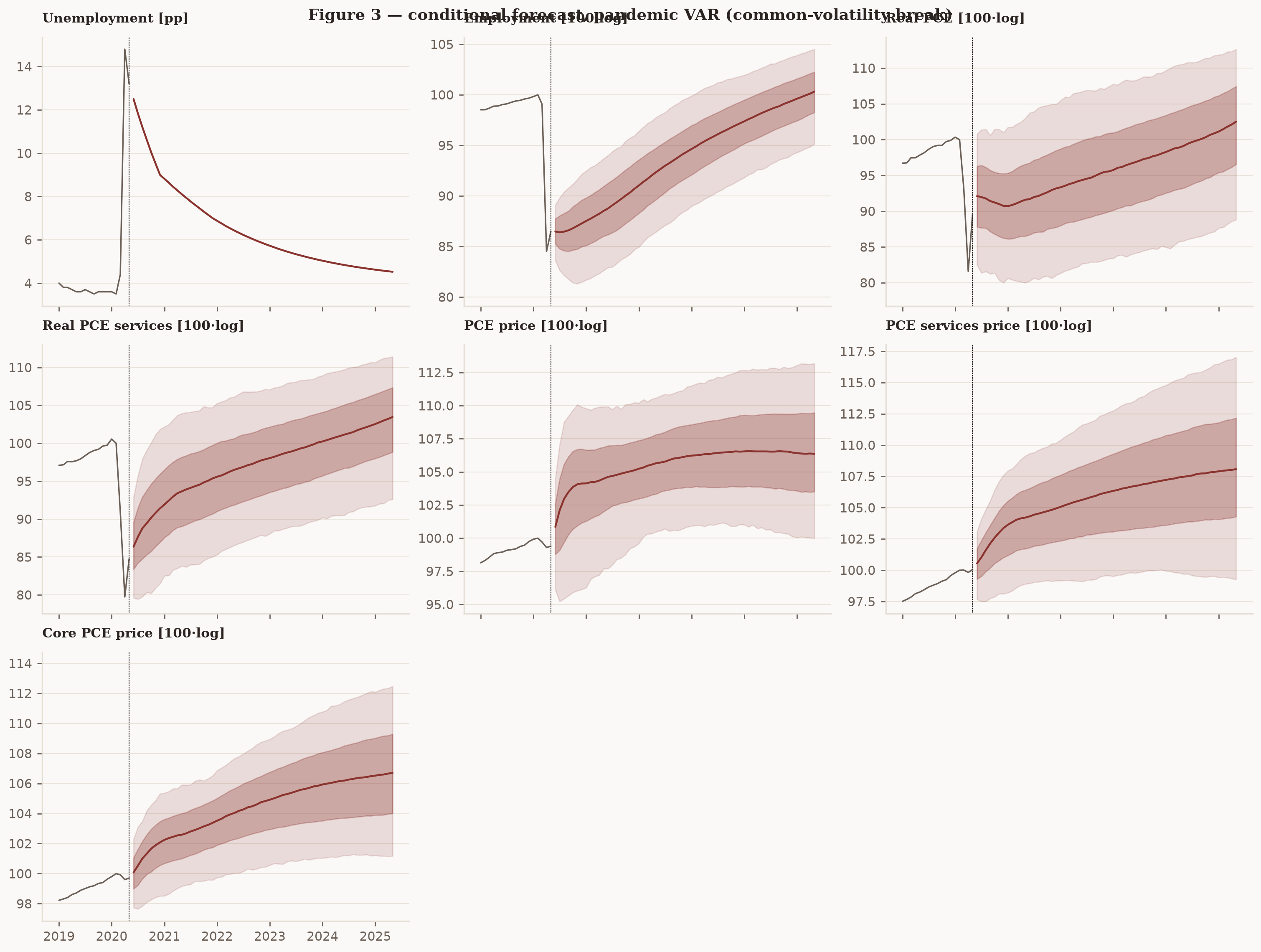
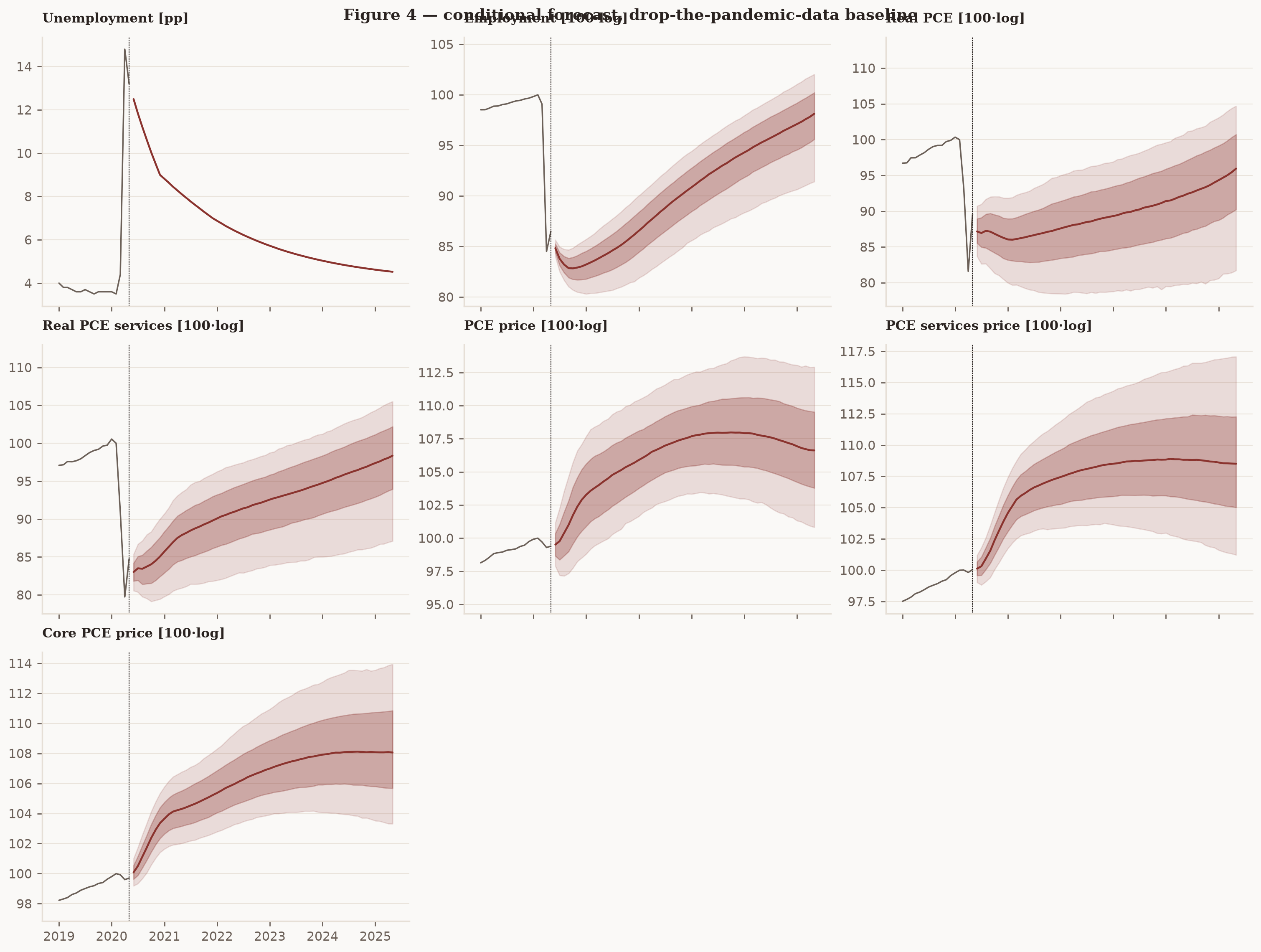
The paper’s headline application is a conditional forecast: fix the future path of unemployment and ask what the model implies for consumption and prices. Both models are seeded from the same history — the thirteen months ending in May 2020 — and conditioned on the same imposed unemployment path. Only the estimated coefficients \(\beta\) and covariance \(\Sigma\) differ between them, so any difference in the forecasts is attributable to how each model treated the pandemic observations, not to different inputs.

We reconstruct a 60-month unemployment path from June 2020 to May 2025. From May 2020’s rate it interpolates (log-linearly) down to 9% by December 2020, then to 7% by December 2021 — a slow-recovery profile in the spirit of the mid-2020 consensus. After 2021 it follows a smooth exponential glide toward a long-run 4%. That post-2021 tail is an extrapolation, not a Blue Chip survey path.

u_may = float(model_df["unemployment"].loc["2020-05-01"])
forecast_index = pd.date_range("2020-06-01", periods=60, freq="MS")
# Month counter from the May-2020 origin: June 2020 is month 1, May 2025 is month 60.
month = np.arange(1, 61)
m_dec2020, m_dec2021 = 7, 19  # months from May 2020 to those December anchors

unemployment_path = np.empty(60)
seg1 = month <= m_dec2020
unemployment_path[seg1] = u_may * (9.0 / u_may) ** (month[seg1] / m_dec2020)
seg2 = (month > m_dec2020) & (month <= m_dec2021)
unemployment_path[seg2] = 9.0 * (7.0 / 9.0) ** ((month[seg2] - m_dec2020) / (m_dec2021 - m_dec2020))
seg3 = month > m_dec2021  # extrapolation beyond December 2021
r = (3.0 / 5.0) ** (1.0 / 12.0)  # annual factor 3/5; 4 + 5·r^m glides from 9 (Dec-20) toward 4
unemployment_path[seg3] = 4.0 + 5.0 * r ** (month[seg3] - m_dec2020)

i_dec2020 = forecast_index.get_loc(pd.Timestamp("2020-12-01"))
i_dec2021 = forecast_index.get_loc(pd.Timestamp("2021-12-01"))
assert abs(unemployment_path[i_dec2020] - 9.0) < 1e-9, "December 2020 anchor must be 9%"
assert abs(unemployment_path[i_dec2021] - 7.0) < 1e-9, "December 2021 anchor must be 7%"

history = model_df.to_numpy()[-13:]
cf_pandemic = conditional_forecast(fitted, history, unemployment_path, index=0, seed=0)
cf_baseline = conditional_forecast(fitted_base, history, unemployment_path, index=0, seed=0)

The headline: how wide are the bands?

The clearest single number is the width of the 95% credible band for real total consumption twelve months out (May 2021). The pandemic model keeps the outbreak months but discounts them through the elevated-then-decaying volatility, so it carries a little more residual uncertainty into the near-term forecast than the model that simply deletes those months. The ratio below quantifies that gap.

pce_idx = var_names.index("pce")
h12 = 11  # twelfth forecast month: May 2021


def pce_band_width(cf):
    draws = cf[:, :, h12, pce_idx].ravel()
    lo, hi = np.quantile(draws, [0.025, 0.975])
    return hi - lo


w_pandemic = pce_band_width(cf_pandemic)
w_baseline = pce_band_width(cf_baseline)
print(f"12-month real-PCE 95% band width — pandemic: {w_pandemic:.2f}, baseline: {w_baseline:.2f}")
print(f"width ratio (pandemic / baseline): {w_pandemic / w_baseline:.2f}")
if not ci:
    assert w_pandemic > w_baseline, "expected the pandemic model's near-term band to be wider than the drop-data baseline"

12-month real-PCE 95% band width — pandemic: 22.97, baseline: 13.39
width ratio (pandemic / baseline): 1.71

What was preserved, adapted, and left open

Preserved. The economic content of Lenza and Primiceri [2022] carries over intact: the seven-variable panel, 13 monthly lags, the natural-conjugate Minnesota prior with an estimated tightness, and — the core idea — a single common volatility scale that spikes in March–May 2020 and decays back to normal, leaving the correlation structure of the shocks untouched.

Adapted. Two inputs differ from the original. The data are a current FRED vintage rather than the 2020 real-time release, so the estimated scales sit near but not on the paper’s values. The conditioning path is reconstructed: a consensus-style slow recovery through 2021, then a labelled extrapolation, in place of the proprietary Blue Chip trajectory.

Left open. The Cholesky responses in Figure 2 are descriptive summaries, not identified structural effects — a genuine structural analysis would need an identification scheme the recursive ordering does not provide. And the decay \(\rho\) is essentially prior-driven: three months of pandemic data fix how large the shocks were without pinning down how quickly volatility returns to normal. A longer post-2020 sample would sharpen it.

References

The work reproduced here is collected on the project bibliography page.