Model Checks and Validation#
A fitted model is a claim, and every claim deserves an audit. This tutorial walks the full checking workflow on real U.S. macroeconomic data: pretest the data before specifying the model, check the prior before sampling, check the sampler after it runs, and check the fitted model against the data it was fitted to. The sequence follows the Bayesian workflow described by Gelman et al. [2020] and Gabry et al. [2019] — each step is cheap, and each one catches a different way of being wrong.
Two how-to guides cover the same APIs in reference form: Testing for Stationarity and Cointegration and Prior and Posterior Predictive Checks. This tutorial shows what running them on genuine data looks like, including the parts where the answers are messy.
The stationarity pretests need the diagnostics extra
(pip install "impulso[diagnostics]"), which pulls in statsmodels.
import arviz as az
import matplotlib.pyplot as plt
import numpy as np
import pandas as pd
from qc_core import plotting

from impulso import (
    VAR,
    VARData,
    adf_test,
    integration_order,
    johansen_test,
    kpss_test,
    select_lag_order,
)
from impulso.samplers import NUTSSampler

plotting.use_ledger_style()
The data#
We reuse the three-variable U.S. monetary policy system from the
Monetary Policy Analysis tutorial: industrial production (output)
and the consumer price index (prices), both entering as \(100 \times \log\), and the
effective federal funds rate (rate) in percentage points. The sample runs from January
1965 to December 2007 — monthly data, 516 observations. That tutorial explains why these
variables and this sample; here they are simply a realistic test bed, with all the
awkwardness real macro data brings.
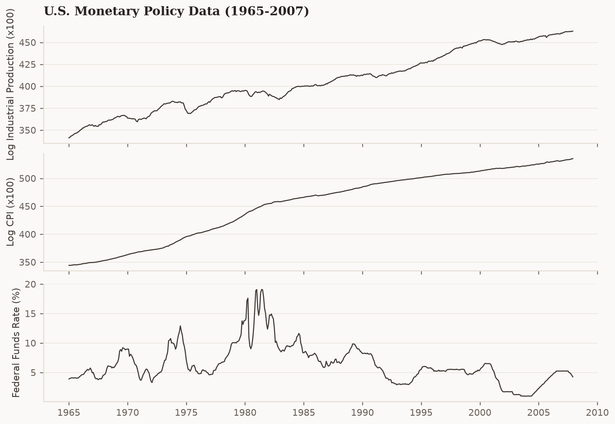
Fig. 8 The three series. Output and prices trend strongly upward; the funds rate is bounded but highly persistent.#
data = VARData.from_df(df, endog=["output", "prices", "rate"])
Step 1: pretest the data#
A VAR in levels and a VAR in differences answer different questions, and the choice should be made deliberately. The pretests report; they do not decide — the modelling decision at the end of this section is ours.
Unit-root tests#
The Augmented Dickey-Fuller test (Dickey and Fuller [1979]) takes a unit root as its null,
so a small p-value argues for stationarity. Because output and prices trend visibly, we
allow a linear trend under the alternative with regression="ct" — testing a trending
series against a constant-only alternative would stack the deck towards non-stationarity.
adf = adf_test(data, regression="ct")
adf.summary()
| statistic | pvalue | lags | crit_1pct | crit_5pct | crit_10pct | reject | conclusion | |
|---|---|---|---|---|---|---|---|---|
| variable | ||||||||
| output | -3.778440 | 0.017684 | 9 | -3.976774 | -3.419202 | -3.132175 | True | stationary |
| prices | -1.129292 | 0.924016 | 13 | -3.976918 | -3.419272 | -3.132216 | False | non-stationary |
| rate | -3.642365 | 0.026444 | 16 | -3.977028 | -3.419325 | -3.132248 | True | stationary |
ADF rejects a unit root for output and rate at the 5% level, but not for prices.
The KPSS test (Kwiatkowski et al. [1992]) flips the burden of proof: its null is stationarity, so a rejection argues for a unit root. Running both is standard practice precisely because ADF has poor power against persistent-but-stationary alternatives.
kpss = kpss_test(data, regression="ct")
kpss.summary()
| statistic | pvalue | lags | crit_1pct | crit_2_5pct | crit_5pct | crit_10pct | pvalue_bounded | reject | conclusion | |
|---|---|---|---|---|---|---|---|---|---|---|
| variable | ||||||||||
| output | 0.219643 | 0.01 | 15 | 0.216 | 0.176 | 0.146 | 0.119 | True | True | non-stationary |
| prices | 0.781241 | 0.01 | 15 | 0.216 | 0.176 | 0.146 | 0.119 | True | True | non-stationary |
| rate | 0.384686 | 0.01 | 15 | 0.216 | 0.176 | 0.146 | 0.119 | True | True | non-stationary |
KPSS rejects stationarity for all three series — note the pvalue_bounded column: the
reported p-values sit at the edge of the published lookup table, so they are bounds, not
estimates. The two tests now disagree on output and rate. That is not a malfunction; it
is the classic signature of highly persistent series in a finite sample, where “unit root”
and “root of 0.98” are close to observationally equivalent. What to do when the tests
disagree is a topic of its own — see
Stationarity pitfalls for a worked discussion.
Integration order#
integration_order automates the difference-and-retest loop, with ADF driving the stopping
rule and KPSS recorded alongside as a cross-check:
order: {'output': 0, 'prices': 2, 'rate': 0}
d_max: 2
inconclusive: ['output', 'prices', 'rate']
| adf_stat | adf_pvalue | adf_lags | adf_reject | kpss_stat | kpss_pvalue | kpss_lags | kpss_reject | kpss_pvalue_bounded | joint_status | ||
|---|---|---|---|---|---|---|---|---|---|---|---|
| variable | d | ||||||||||
| output | 0 | -3.778440 | 1.768423e-02 | 9 | True | 0.219643 | 0.010000 | 15 | True | True | conflicting |
| prices | 0 | -1.129292 | 9.240160e-01 | 13 | False | 0.781241 | 0.010000 | 15 | True | True | unit_root |
| 1 | -2.775570 | 6.184899e-02 | 12 | False | 1.061279 | 0.010000 | 14 | True | True | unit_root | |
| 2 | -7.628023 | 2.043913e-11 | 13 | True | 0.500000 | 0.041667 | 513 | True | False | conflicting | |
| rate | 0 | -3.642365 | 2.644435e-02 | 16 | True | 0.384686 | 0.010000 | 15 | True | True | conflicting |
Every variable lands on the inconclusive list, each for an instructive reason:
outputandratestop at \(d = 0\) withjoint_status = "conflicting"— both tests reject, which is the ADF/KPSS disagreement from above.pricesfails to reject a unit root even in first differences at \(\alpha = 0.05\) (monthly inflation is itself very persistent) and only stops at \(d = 2\). Whether the price level is I(1) or I(2) is a genuinely unsettled question in the unit-root literature, and a 43-year sample does not settle it either.
The honest summary: prices is clearly non-stationary, output and rate are too
persistent to classify cleanly. Treat the order numbers as a table to read, not a verdict
to obey.
Cointegration#
If the series are individually non-stationary they may still share long-run relationships,
in which case differencing every series would throw those relationships away. The Johansen
procedure (Johansen [1991]) estimates how many such relationships exist. It needs a
lag order first — k_ar_diff counts lagged differences, so it is \(p - 1\) for a VAR(\(p\))
in levels:
AIC selects 11, BIC selects 2, HQ selects 3
rank (trace): 2, rank (max eigenvalue): 2
| trace_stat | trace_crit | trace_reject | maxeig_stat | maxeig_crit | maxeig_reject | |
|---|---|---|---|---|---|---|
| r | ||||||
| 0 | 75.026925 | 29.7961 | True | 57.355524 | 21.1314 | True |
| 1 | 17.671401 | 15.4943 | True | 14.500860 | 14.2639 | True |
| 2 | 3.170542 | 3.8415 | False | 3.170542 | 3.8415 | False |
The criteria disagree in their usual pattern — AIC generous at 11, BIC parsimonious at 2 — and we take Hannan-Quinn’s compromise of 3 lags. Both Johansen statistics then agree on a cointegration rank of 2: two long-run relationships tie the three series together, leaving a single common stochastic trend.
The decision: fit in levels#
Three facts point the same way. The series are non-stationary or nearly so; they are cointegrated, so differencing everything would discard the long-run structure; and Sims et al. [1990] showed that Bayesian inference in a levels VAR is valid whether or not unit roots are present. The Minnesota prior (Doan et al. [1984]) is built for exactly this situation — it shrinks each equation towards a random walk, which is a good description of these series. So: a VAR(3) in levels with a Minnesota prior.
spec = VAR(lags=3, prior="minnesota")
Step 2: check the prior before sampling#
A prior predictive check asks whether the model before seeing the likelihood can produce
data on the same planet as the data we have (Gelman et al. [1996];
Gabry et al. [2019]). VAR.prior_predictive draws from exactly the graph fit will
sample, so there is no risk of checking a different prior than the one we use:
prior = spec.prior_predictive(data, draws=500, random_seed=0)
axes = az.plot_ppc(prior, group="prior", num_pp_samples=50, coords={"var": ["rate"]})
Sampling: [B, intercept, obs, sigma_sd, tril_offdiag]
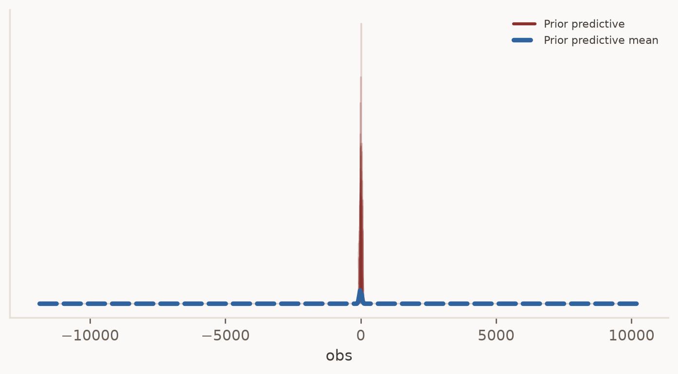
The pooled density for the funds rate shows the prior band comfortably containing the observed distribution, without being absurdly wider. A quantile coverage check makes that quantitative across all three variables. Quantiles, not mean \(\pm k \cdot\) sd: the default scale prior is HalfCauchy, which has no finite moments, so a prior predictive mean is meaningless — see the predictive-checks how-to.
prior_draws = prior.prior_predictive["obs"].values[0]  # (draws, time, var)
lower, upper = np.quantile(prior_draws, [0.025, 0.975], axis=0)
observed = prior.observed_data["obs"].values

coverage = ((observed >= lower) & (observed <= upper)).mean()
width = np.median(upper - lower)
print(
    f"95% prior band covers {coverage:.1%} of the data; median band width {width:.0f}"
)
95% prior band covers 100.0% of the data; median band width 210
Full coverage, with a band roughly 210 units wide against series that span roughly 1 to
535. The prior is loose — as a shrinkage prior should be — but not so diffuse that it burns
sampling effort in absurd regions. If the band had excluded chunks of the data, the prior
would be fighting the likelihood, and we would revisit the Minnesota hyperparameters before
spending a single MCMC second (see
The Minnesota Prior, From Scratch for tuning tightness).
Step 3: fit, then interrogate the sampler#
fit samples the posterior with NUTS, the adaptive Hamiltonian Monte Carlo variant of
Hoffman and Gelman [2014]. HMC is efficient, and — just as valuable — it is loud when it
fails: its diagnostics flag problems that would pass silently in older samplers
(Betancourt [2017]). Loud only helps if you listen, so after every fit we check, in
order: divergences, \(\widehat{R}\), effective sample size, and the energy diagnostic.
We start with production-scale settings and default mass-matrix adaptation:
if ci:
    sampler = NUTSSampler(
        draws=50, tune=500, chains=2, cores=1, target_accept=0.9, random_seed=123
    )
else:
    sampler = NUTSSampler(
        draws=1500,
        tune=1500,
        chains=4,
        cores=4,
        target_accept=0.9,
        random_seed=123,
        nuts_sampler="nutpie",
    )

fitted = spec.fit(data, sampler=sampler)
Smoke renders
In CI this notebook runs with drastically shrunk MCMC (IMPULSO_DOCS_CI=1), so the printed
diagnostics in a smoke build are not representative. The narrative describes the
full-fidelity render.
Divergences#
A divergence is a numerical failure of the leapfrog integrator, and it is the sharpest signal HMC emits: divergences concentrate exactly where the posterior has geometry the sampler cannot traverse, so the affected region is under-explored and estimates that pass through it are biased (Betancourt [2017]). Zero is the only acceptable count:
None — but zero divergences is necessary, not sufficient. The next checks catch failures that never trip the integrator.
\(\widehat{R}\) and effective sample size#
az.summary(kind="diagnostics") reports, per parameter:
r_hat— the rank-normalised split-\(\widehat{R}\) of Vehtari et al. [2021], the modern refinement of Gelman and Rubin [1992]. It compares within-chain and between-chain variance; at convergence it is 1, and values above 1.01 mean the chains have not agreed on what the posterior looks like.ess_bulk— the effective number of independent draws for the centre of the posterior, which governs how well means and medians are estimated.ess_tail— the same for the 5% and 95% quantiles, which governs credible-interval endpoints. A chain can estimate the centre well and the tails badly.mcse_mean/mcse_sd— the Monte Carlo standard error those ESS values imply.
Vehtari et al. [2021] recommend at least 400 effective draws (100 per chain on four chains) before trusting the estimates. Rather than eyeball hundreds of rows, filter for violations:
16 of 57 parameters flagged
| mcse_mean | mcse_sd | ess_bulk | ess_tail | r_hat | |
|---|---|---|---|---|---|
| B[prices, L2.prices] | 0.010 | 0.004 | 18.0 | 44.0 | 1.19 |
| B[prices, L1.prices] | 0.006 | 0.002 | 26.0 | 105.0 | 1.18 |
| B[prices, L3.prices] | 0.004 | 0.002 | 33.0 | 63.0 | 1.10 |
| B[prices, L2.output] | 0.003 | 0.001 | 31.0 | 49.0 | 1.10 |
| B[prices, L1.output] | 0.002 | 0.001 | 46.0 | 290.0 | 1.07 |
| B[prices, L3.output] | 0.001 | 0.000 | 96.0 | 359.0 | 1.04 |
| B[output, L2.prices] | 0.002 | 0.001 | 156.0 | 475.0 | 1.04 |
| B[output, L1.prices] | 0.002 | 0.001 | 163.0 | 431.0 | 1.03 |
The fit fails the check. In the full render, \(\widehat{R}\) reaches 1.13 with bulk ESS in
the low dozens, and the flagged rows are not random: they concentrate in the prices
equation’s own lags (B[prices, L1.prices], L2.prices, L3.prices) and their
neighbours. A trace plot shows what that means in the raw draws — the four chains disagree
about the coefficient’s location and wander slowly within it, instead of overlapping as
indistinguishable noise:
az.plot_trace(
    fitted.idata,
    var_names=["B"],
    coords={"var": ["prices"], "coeff": ["L1.prices", "L2.prices"]},
)
array([[<Axes: title={'left': 'B'}>, <Axes: title={'left': 'B'}>]],
      dtype=object)

The energy diagnostic#
az.plot_energy overlays the distribution of the Hamiltonian energy with the distribution
of its step-to-step changes; when the two differ badly (Bayesian fraction of missing
information, BFMI, below about 0.3) the sampler cannot move between energy levels fast
enough to explore the tails (Betancourt [2017]):
az.plot_energy(fitted.idata)
<Axes: >
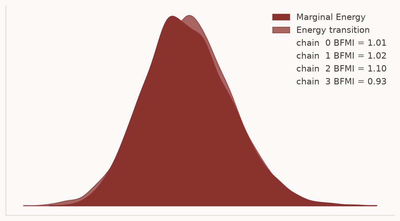
The two distributions overlap and BFMI is near 1 — this check passes. That is the point of running the checks as a battery: divergences and energy are clean while \(\widehat{R}\) and ESS fail, and only the full battery tells you the problem is slow mixing rather than pathological geometry.
Fixing it#
Why does mixing fail here? The regressors of a levels VAR are lagged copies of
near-random-walk series — prices at lags one, two, and three are almost the same
variable. Individually each coefficient is weakly identified even though their sum is
well determined, so the posterior has long, narrow, correlated ridges, and NUTS’s default
diagonal mass matrix cannot be scaled to match. This is a known pathology of large
VARs, and nutpie ships a remedy: a low-rank modified mass matrix that adapts to exactly
this kind of ill-conditioning.
if ci:
    sampler = NUTSSampler(
        draws=50,
        tune=500,
        chains=2,
        cores=1,
        target_accept=0.9,
        random_seed=123,
        nuts_sampler_kwargs={"low_rank_modified_mass_matrix": True},
    )
else:
    sampler = NUTSSampler(
        draws=1500,
        tune=1500,
        chains=4,
        cores=4,
        target_accept=0.9,
        random_seed=123,
        nuts_sampler="nutpie",
        nuts_sampler_kwargs={"low_rank_modified_mass_matrix": True},
    )

fitted = spec.fit(data, sampler=sampler)

summ = az.summary(fitted.idata, kind="diagnostics")
flagged = summ[(summ["r_hat"] > 1.01) | (summ["ess_bulk"] < 400)]
print(f"divergences: {int(fitted.idata.sample_stats.diverging.sum())}")
print(f"{len(flagged)} of {len(summ)} parameters flagged")
print(
    f"max r_hat: {summ['r_hat'].max():.3f}, min ess_bulk: {summ['ess_bulk'].min():.0f}"
)
divergences: 0
0 of 57 parameters flagged
max r_hat: 1.000, min ess_bulk: 5945
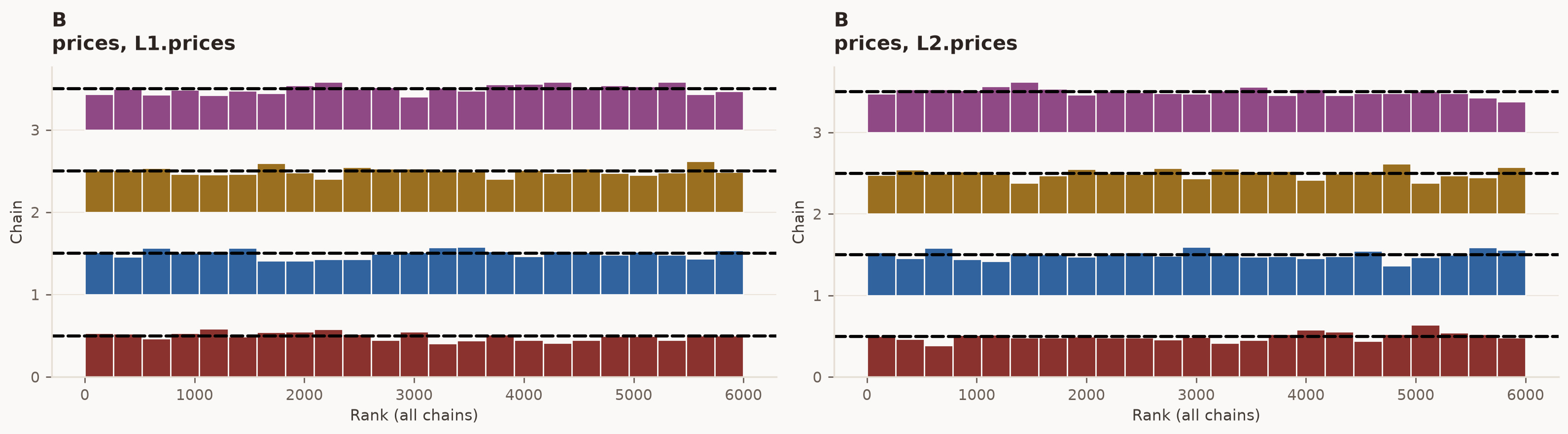
In the full render every flag clears: no divergences, \(\widehat{R} = 1.00\) throughout, and a minimum bulk ESS in the thousands. A rank plot — Vehtari et al. [2021]’s preferred convergence visual — confirms it on the previously worst coefficient. When chains mix, each chain’s draws are spread uniformly across the pooled ranking, so all histograms should look flat:
az.plot_rank(
    fitted.idata,
    var_names=["B"],
    coords={"var": ["prices"], "coeff": ["L1.prices", "L2.prices"]},
)
array([<Axes: title={'left': 'B\nprices, L1.prices'}, xlabel='Rank (all chains)', ylabel='Chain'>,
       <Axes: title={'left': 'B\nprices, L2.prices'}, xlabel='Rank (all chains)', ylabel='Chain'>],
      dtype=object)
Going deeper
This section covers the checks you should never skip. For the full menu — MCSE-aware reporting, chain-splitting subtleties, folded \(\widehat{R}\) — see the ArviZ API reference (Kumar et al. [2019]), Vehtari et al. [2021], and Betancourt [2017].
Step 4: check the fit against the data#
The sampler converged; now, did it converge to a model worth having? A posterior predictive
check replicates the estimation sample from the posterior and compares the replicates with
what actually happened (Gelman et al. [1996]). Each replicate is one-step-ahead
conditioned on the observed lags — the standard predictive object for a conditional model,
and the one az.plot_ppc expects:
ppc = fitted.posterior_predictive(seed=0)
axes = az.plot_ppc(ppc, num_pp_samples=100, coords={"var": ["rate"]})
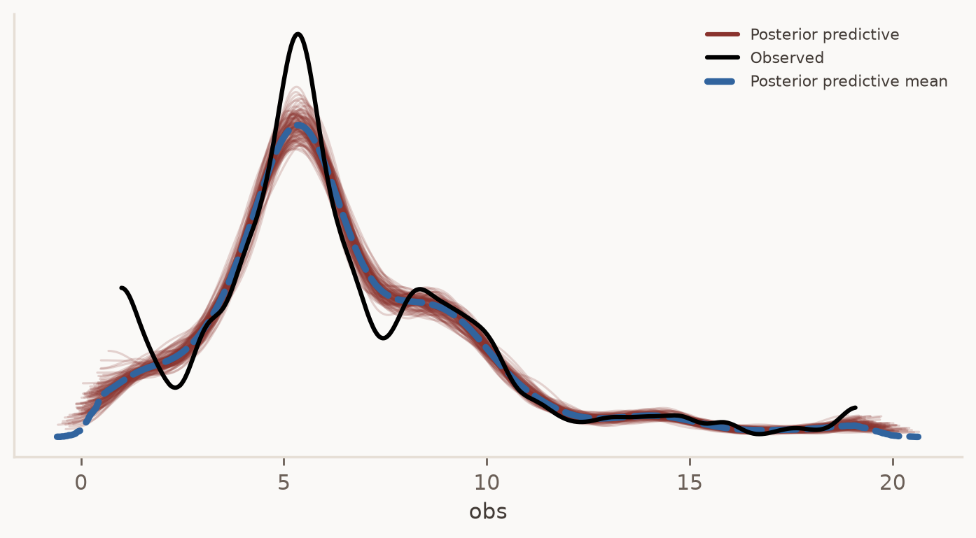
The replicate densities track the observed density closely — compare with the prior predictive version of this plot above, where the band was hundreds of units wide. The same quantile coverage check, now on the posterior:
rep = ppc.posterior_predictive["obs"].values  # (chain, draw, time, var)
flat = rep.reshape(-1, *rep.shape[2:])  # (chain*draw, time, var)
lower, upper = np.quantile(flat, [0.025, 0.975], axis=0)
observed = ppc.observed_data["obs"].values

pooled = ((observed >= lower) & (observed <= upper)).mean()
per_var = ((observed >= lower) & (observed <= upper)).mean(axis=0)
print(f"95% band covers {pooled:.1%} of observations")
for name, cov in zip(data.endog_names, per_var, strict=True):
    print(f"  {name}: {cov:.1%}")
95% band covers 95.2% of observations
  output: 94.5%
  prices: 94.9%
  rate: 96.1%
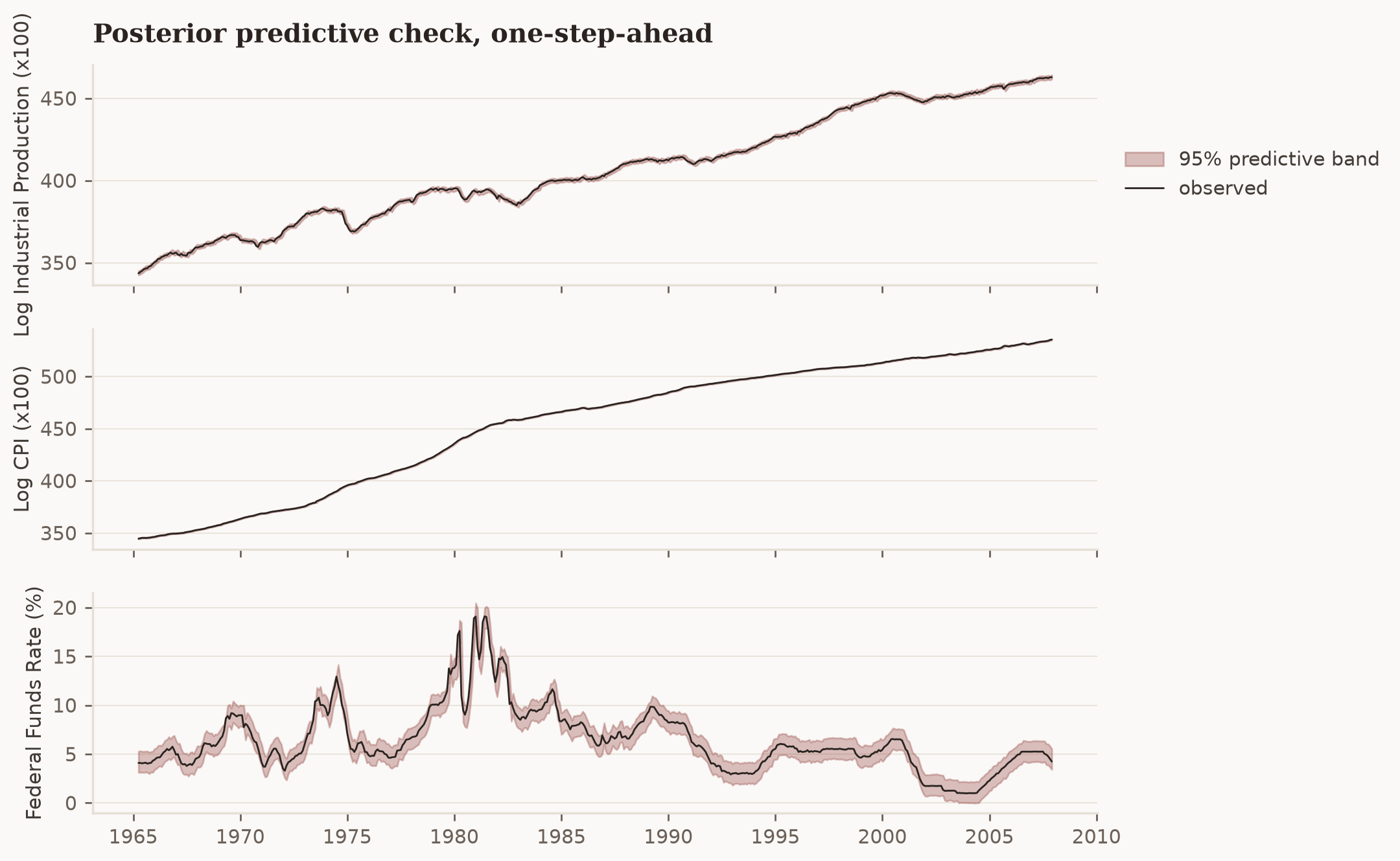
Fig. 9 Observed series against the 95% posterior predictive band. The band is one-step-ahead, so it hugs the data; the check is whether the right fraction of points escape it.#
In the full render the band covers about 95% of observations overall and per variable — the model is neither over-confident (coverage well below 95%) nor over-dispersed (coverage near 100%). One caveat worth carrying forward: the covariance here is constant through time, while the funds-rate panel visibly is not — the early-1980s Volcker period strains the band. The Stochastic Volatility tutorial relaxes exactly that assumption.
For residual diagnostics — subtracting the conditional mean under parameter uncertainty via
posterior_predictive(simulate_innovations=False) — and for attaching the replicates to
fitted.idata, see the predictive-checks how-to.
The checklist#
When |
Question |
Tool |
|---|---|---|
Before specifying |
Levels or differences? Shared trends? |
|
Before sampling |
Can the prior produce plausible data? |
|
After sampling |
Did the sampler explore the posterior? |
divergences, |
After sampling |
Does the model reproduce the sample? |
|
None of these checks proves the model right; each can prove it wrong cheaply. Run all four before you forecast, identify shocks, or hand results to anyone.
What’s next#
Forecast with the checked model — the Forecasting tutorial
Identify structural shocks — the Structural Analysis tutorial
Time-varying volatility, for the constant-covariance caveat above — the Stochastic Volatility tutorial
We currently have some availability for consulting on how Bayesian modelling, vector autoregressions, and impulso can be integrated into your team's macroeconomic and financial forecasting work. If this sounds relevant, book an introductory call. These calls are for consulting inquiries only. For technical usage questions and free community support, please use GitHub Discussions and the documentation.