The Minnesota Prior, From Scratch

Every Bayesian VAR in Impulso ships with prior="minnesota" switched on by default. This tutorial explains what that default is doing to your model: the arithmetic behind it, the three numbers you can turn, and what each one costs you.

It assumes you know what a VAR is and have seen a normal distribution. It does not assume you have met a Minnesota prior before. If you want the compressed reference version instead, read the Minnesota prior explanation.

import matplotlib.pyplot as plt
import numpy as np
import pandas as pd
from qc_core import plotting

from impulso import VAR, MinnesotaPrior, VARData
from impulso.samplers import NUTSSampler

plotting.use_ledger_style()

The problem: a VAR runs out of data fast

A VAR with \(n\) variables and \(p\) lags has \(n^2 p\) slope coefficients plus \(n\) intercepts. The quadratic term is the trouble. Adding one variable to a 5-variable VAR(4) adds 44 slope coefficients, not 4. Meanwhile the sample gives you \(nT\) numbers to estimate them from, which grows only linearly.

Fig. 1 plots both sides for a quarterly sample of \(T = 200\), roughly fifty years of data — about as long a macroeconomic series as you will ever be handed.

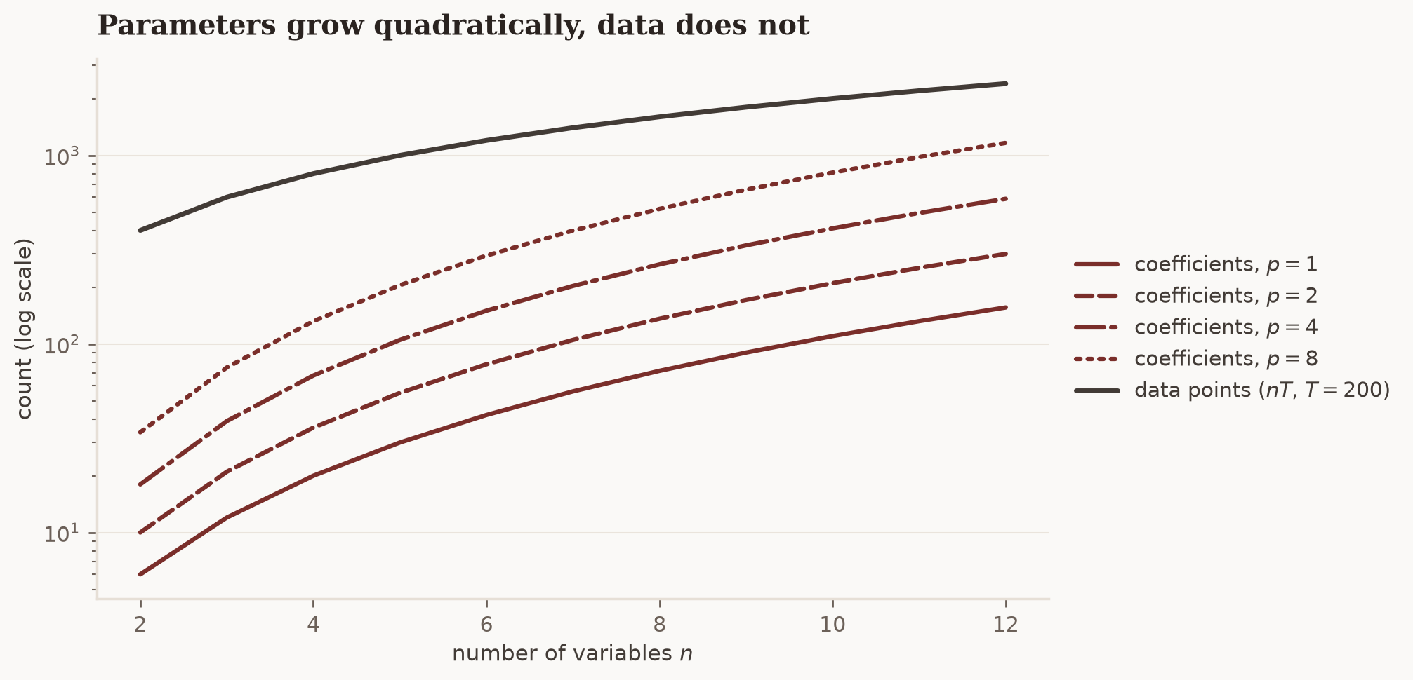
Fig. 1 Free VAR coefficients against available data points for a sample of \(T = 200\). The parameter count grows quadratically in the number of variables; the data does not.

An 8-variable VAR(8) has 520 coefficients against 1,600 data points. Ordinary least squares will happily fit it, and the fit will be mostly noise: the estimates have enormous sampling variance, and the implied dynamics are frequently explosive. This is the curse of dimensionality that Sims [1980] flagged in the paper that introduced VARs to macroeconomics, and it is the reason Doan et al. [1984] and Litterman [1986] — then at the Federal Reserve Bank of Minneapolis and the University of Minnesota — proposed fixing it with a prior rather than with more data.

The idea: start from a random walk

Write the VAR in the form Impulso estimates:

(1)\[ y_t = c + \sum_{l=1}^{p} A_l\, y_{t-l} + u_t, \qquad u_t \sim \mathcal{N}(0, \Sigma) \]

where \(y_t \in \mathbb{R}^n\) and each \(A_l\) is \(n \times n\). Stack the lag matrices side by side into the single coefficient matrix Impulso samples,

(2)\[ B = \begin{bmatrix} A_1 & A_2 & \cdots & A_p \end{bmatrix} \in \mathbb{R}^{n \times np}, \]

and write \(\beta_{ij}^{(l)}\) for the entry of \(A_l\) in row \(i\), column \(j\): the response of variable \(i\) to lag \(l\) of variable \(j\).

The Minnesota prior is a normal distribution on every one of these entries, treated as independent:

(3)\[ \beta_{ij}^{(l)} \sim \mathcal{N}\!\left( m_{ij}^{(l)},\; \big(s_{ij}^{(l)}\big)^2 \right). \]

All the content is in how \(m\) and \(s\) are chosen. The mean encodes a guess; the standard deviation encodes how strongly you hold it.

The mean: each series is a random walk

The guess is that every variable is a random walk and nothing predicts anything else:

(4)\[\begin{split} m_{ij}^{(l)} = \begin{cases} 1 & \text{if } i = j \text{ and } l = 1, \\ 0 & \text{otherwise.} \end{cases} \end{split}\]

So \(A_1\) has ones on its diagonal, and every other coefficient in the model is centred at zero. Two things motivate this. Macroeconomic levels — output, prices, employment — really are close to unit-root processes, and a random walk is a famously hard forecast to beat at short horizons. And it is a safe default: shrinking toward it removes cross-variable dynamics rather than inventing them, so the prior can only cost you predictability you had real evidence for.

Working with growth rates or anomalies?

The random-walk mean is a statement about levels. If you have already differenced, de-meaned, or standardised your series, a prior mean of one on the own first lag is too persistent — the honest centre is closer to zero. You can still use MinnesotaPrior, but the shrinkage target is then working against you rather than for you. Write a custom prior with a zero mean instead (see Writing a Custom Prior); it is a ten-line class.

The standard deviation: three knobs

The prior mean above is deliberately naive. What stops it from dominating the data is the standard deviation, and this is where the tuning happens:

(5)\[\begin{split} s_{ij}^{(l)} = \underbrace{\lambda}_{\text{tightness}} \times \underbrace{d(l)}_{\text{lag decay}} \times \underbrace{\begin{cases} 1 & i = j \\ \kappa & i \neq j \end{cases}}_{\text{cross shrinkage}}, \qquad d(l) = \begin{cases} 1/l & \texttt{"harmonic"} \\ 1/l^{2} & \texttt{"geometric"}. \end{cases} \end{split}\]

Read the three factors as three separate beliefs:

Factor	Argument	Default	The belief it encodes
\(\lambda\)	tightness	0.1	How far any coefficient may stray from its prior mean. \(\lambda \to 0\) freezes the model at the random walk; \(\lambda \to \infty\) recovers OLS.
\(d(l)\)	decay	"harmonic"	Distant lags matter less than recent ones, so they get shrunk harder.
\(\kappa\)	cross_shrinkage	0.5	A variable’s own history is more informative about it than other variables’ histories. \(\kappa = 0\) forbids cross-variable dynamics entirely; \(\kappa = 1\) treats own and cross lags alike.

That is the whole prior. MinnesotaPrior.build_priors returns exactly Eq. 4 and Eq. 5 as two arrays, B_mu and B_sigma, which VAR.fit hands straight to PyMC as the mean and standard deviation of a normal prior on B.

prior = MinnesotaPrior()  # tightness=0.1, decay="harmonic", cross_shrinkage=0.5
params = prior.build_priors(n_vars=3, n_lags=4)
{k: v.shape for k, v in params.items()}

{'B_mu': (3, 12), 'B_sigma': (3, 12)}

Seeing the prior

Those two \(3 \times 12\) arrays are the prior, so plotting them is the most direct way to understand it. Rows are equations (which variable is being explained); columns run over the 12 regressors in lag-major order — all three variables at lag 1, then all three at lag 2, and so on.

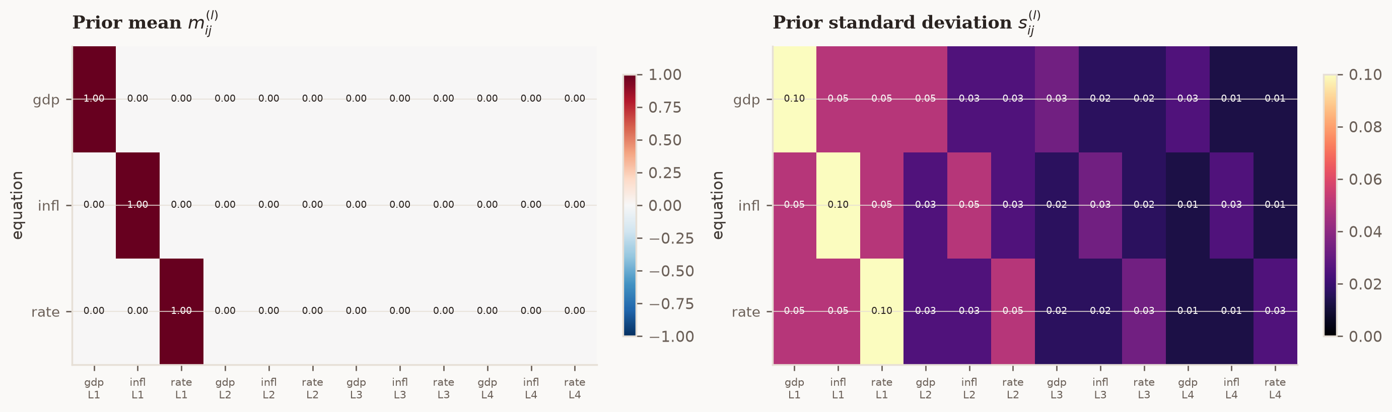
Fig. 2 The default Minnesota prior for a 3-variable VAR(4), shown as the two arrays Impulso actually passes to PyMC. Left: prior means — ones on the own first lag, zero everywhere else. Right: prior standard deviations — brightest on own recent lags, dark on distant cross lags.

The left panel is the random walk: a one wherever a variable meets its own first lag, zero everywhere else. The right panel is where the tuning lives. The largest prior standard deviation anywhere in the model is 0.10, on the own first lags — a coefficient the data must fight for even in the most permissive corner of the prior. By lag 4 the own-lag standard deviation is 0.025 and the cross-lag standard deviation is 0.0125, which is effectively a hard zero.

How fast the lags die out

The decay argument controls the slope of that decline. Harmonic decay (\(1/l\)) is gentle enough to leave seasonal or long-cycle dynamics some room; geometric decay (\(1/l^2\)) all but deletes anything past the second lag.

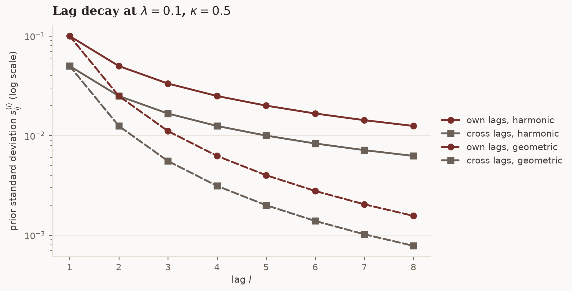
Fig. 3 Prior standard deviation by lag, read out of build_priors for an 8-lag model. Geometric decay reaches near-zero by lag 3; harmonic decay leaves distant lags an order of magnitude more room.

The constant vertical gap between the accent and muted curves is cross_shrinkage: a factor of \(\kappa = 0.5\) applied uniformly across lags. Setting cross_shrinkage=0 collapses the muted curves to zero and turns the VAR into \(n\) independent autoregressions — useful as a forecasting benchmark, useless for structural work, since a variable that cannot respond to another variable’s lags has no dynamic transmission to identify.

What the prior looks like as a distribution

Fig. 4 draws the same information as densities, which is how the sampler sees it. Each curve is the prior on a single coefficient before any data arrives.

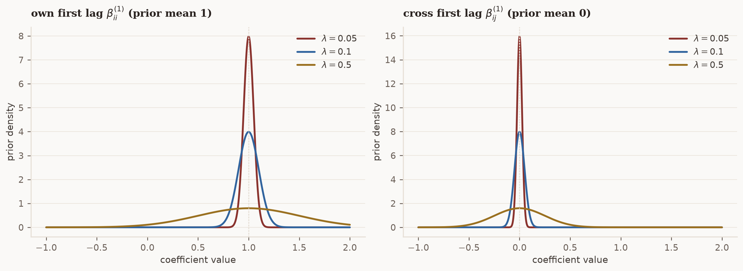
Fig. 4 Prior densities on two representative coefficients at three tightness settings. Left: the own first-lag coefficient, centred on the random walk. Right: a cross-variable first-lag coefficient, centred on zero and additionally shrunk by \(\kappa = 0.5\). The vertical scales are independent — compare the widths.

At \(\lambda = 0.05\) the own first-lag coefficient is confined to roughly \([0.85, 1.15]\) before the data speaks. At \(\lambda = 0.5\) that same coefficient ranges over \([0, 2]\) and the prior has essentially stopped constraining anything.

What the prior believes about the world

Densities on individual coefficients are hard to price. What matters is the dynamics those coefficients imply, and you can look at that directly by drawing \(B\) from the prior and simulating the system forward. This is a prior predictive check, and it costs nothing: no sampler, no data, just the prior arrays and some linear algebra.

The summary statistic to watch is the spectral radius: the largest eigenvalue modulus of the VAR’s companion matrix. Below one, shocks decay and the system is stationary. Above one, shocks compound and the system explodes. Each prior draw of \(B\) gives us one of these numbers.

def companion_matrix(B: np.ndarray, n_vars: int, n_lags: int) -> np.ndarray:
    """Companion form of a VAR coefficient matrix stacked as [A_1 ... A_p]."""
    dim = n_vars * n_lags
    companion = np.zeros((dim, dim))
    companion[:n_vars] = B
    companion[n_vars:, : dim - n_vars] = np.eye(dim - n_vars)
    return companion


def spectral_radius(B: np.ndarray, n_vars: int, n_lags: int) -> float:
    """Largest eigenvalue modulus; < 1 means the VAR is stable."""
    return float(np.abs(np.linalg.eigvals(companion_matrix(B, n_vars, n_lags))).max())


def simulate(B: np.ndarray, n_vars: int, n_lags: int, steps: int, rng: np.random.Generator) -> np.ndarray:
    """Simulate a path from a VAR with unit-variance shocks, starting from zero."""
    y = np.zeros((steps + n_lags, n_vars))
    for t in range(n_lags, steps + n_lags):
        x = np.concatenate([y[t - l] for l in range(1, n_lags + 1)])
        y[t] = B @ x + rng.standard_normal(n_vars)
    return y[n_lags:]

N_VARS, N_LAGS, N_DRAWS = 3, 4, 400
rng = np.random.default_rng(0)
lambdas = [0.05, 0.2, 1.0]

prior_draws = {}
for lam in lambdas:
    pp = MinnesotaPrior(tightness=lam).build_priors(n_vars=N_VARS, n_lags=N_LAGS)
    B_draws = rng.normal(pp["B_mu"], pp["B_sigma"], size=(N_DRAWS, *pp["B_mu"].shape))
    radii = np.array([spectral_radius(B, N_VARS, N_LAGS) for B in B_draws])
    prior_draws[lam] = (B_draws, radii)

pd.DataFrame(
    {
        "tightness": lambdas,
        "median radius": [np.median(prior_draws[lam][1]).round(2) for lam in lambdas],
        "90th pct radius": [np.quantile(prior_draws[lam][1], 0.9).round(2) for lam in lambdas],
        "share above 1.1": [(prior_draws[lam][1] > 1.1).mean().round(2) for lam in lambdas],
    }
).set_index("tightness")

	median radius	90th pct radius	share above 1.1
tightness
0.05	1.05	1.10	0.13
0.20	1.19	1.42	0.72
1.00	1.91	2.88	0.94

Notice where the mass sits. At every tightness the median radius is at or just above one, because the prior mean Eq. 4 is a random walk and a random walk has spectral radius exactly one. The Minnesota prior is deliberately parked on the boundary of stationarity — it is not a stationarity prior, and it never claims to be.

Nor is a bare stability count the right diagnostic here: the largest of several near-unit eigenvalues is biased upward, so most draws come out technically explosive even at tiny \(\lambda\). What matters is by how much. At \(\lambda = 0.05\) only about an eighth of draws exceed a radius of 1.10 — these are near-unit-root systems, which is what macroeconomic levels look like. At \(\lambda = 1.0\) the median draw has radius 1.9, meaning a shock roughly doubles every period. Fig. 5 shows what that difference means for simulated data.

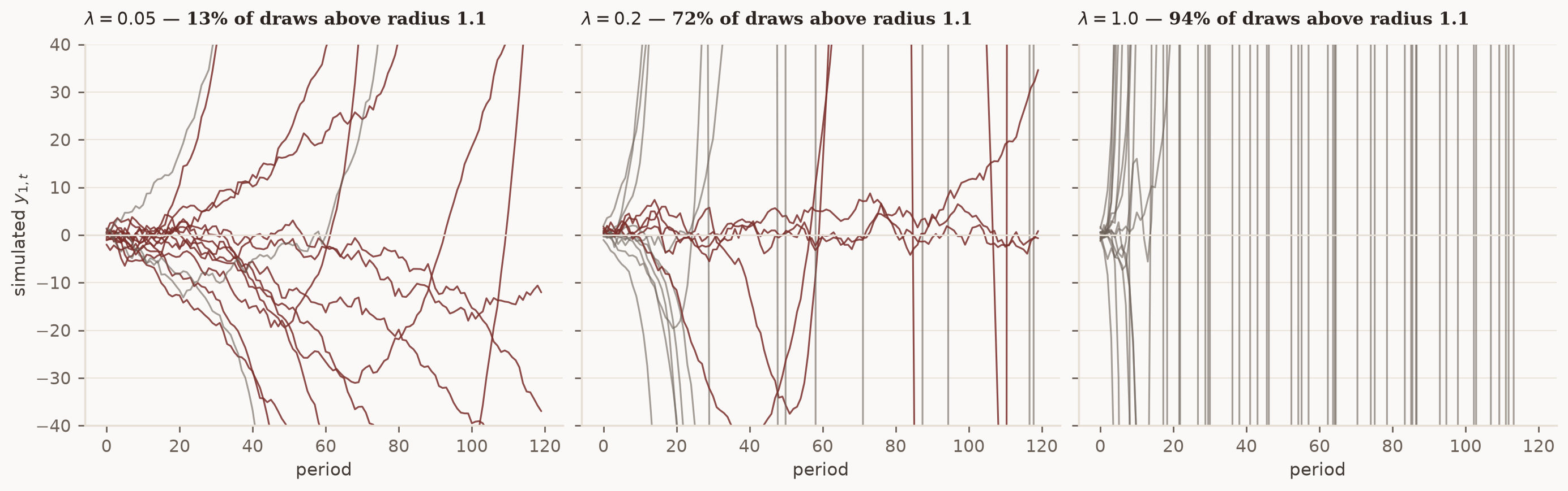
Fig. 5 Prior predictive paths for the first variable of a 3-variable VAR(4), 15 draws per panel, 120 periods each. Accent paths come from draws with spectral radius below 1.1 (near-unit-root); muted paths from more explosive draws, most of which leave the frame within a few periods. Tight shrinkage implies plausible macroeconomic series; loose shrinkage implies almost nothing that resembles data.

This is the argument for shrinkage stated in the units you care about. A loose prior is not “letting the data decide” — it is asserting, before seeing anything, that the economy probably detonates, and the likelihood then has to spend the sample arguing it back down. Tightening \(\lambda\) concentrates prior mass on the wandering, highly persistent behaviour that real macroeconomic levels actually exhibit.

What the prior does to the posterior

Prior predictive plausibility is necessary, not sufficient. The tightest prior is always the most plausible-looking, and it is also useless — set \(\lambda\) small enough and you get back your random walk regardless of what the data says. The real question is the bias–variance trade-off, so let us measure it.

We simulate a 3-variable VAR(1) — persistent, as macroeconomic levels are, with a spectral radius of 0.89 — then deliberately fit a VAR(4), three times more lags than the truth. This is the realistic situation: you do not know \(p\), so you pick generously and rely on the prior to switch off what is not there.

TRUE_A = np.array([
    [0.85, 0.05, -0.15],  # gdp: highly persistent, hurt by last period's rate
    [0.10, 0.80, 0.05],  # inflation: follows gdp, persistent
    [0.05, 0.20, 0.75],  # rate: leans against inflation, persistent
])
T_TRAIN, T_TEST = 100, 60

sim = np.random.default_rng(11)
y = np.zeros((T_TRAIN + T_TEST + 1, 3))
for t in range(1, len(y)):
    y[t] = TRUE_A @ y[t - 1] + sim.standard_normal(3) * 0.5
y_train, y_test_start = y[:T_TRAIN], T_TRAIN

index = pd.date_range("1990-01-01", periods=T_TRAIN, freq="QS")
train_data = VARData(endog=y_train, endog_names=["gdp", "infl", "rate"], index=index)

# True B padded out to VAR(4): lags 2-4 are genuinely zero.
FIT_LAGS = 4
B_true = np.zeros((3, 3 * FIT_LAGS))
B_true[:, :3] = TRUE_A

With only 100 training observations and 39 coefficients to place, this is exactly the regime the Minnesota prior was built for. We fit the same model at six tightness values spanning “almost a random walk” to “almost OLS”.

TIGHTNESS_GRID = [0.02, 0.05, 0.1, 0.25, 0.5, 2.0]
sampler_kwargs = dict(draws=25, tune=25, chains=2, cores=1, random_seed=42) if ci else dict(
    draws=500, tune=500, chains=2, cores=1, random_seed=42
)

posterior_means = {}
for lam in TIGHTNESS_GRID:
    spec = VAR(lags=FIT_LAGS, prior=MinnesotaPrior(tightness=lam))
    fitted = spec.fit(train_data, sampler=NUTSSampler(**sampler_kwargs))
    posterior_means[lam] = (
        fitted.coefficients.mean(axis=(0, 1)),  # (n_vars, n_vars * n_lags)
        fitted.intercepts.mean(axis=(0, 1)),  # (n_vars,)
    )

Two things get measured. Coefficient error is the root mean squared distance between the posterior mean of \(B\) and the truth — available only because we simulated the data. One-step forecast error is the honest out-of-sample version: using each fitted model’s posterior mean, predict every one of the 60 held-out periods from its actual predecessors and compare against what happened.

def one_step_rmse(B: np.ndarray, c: np.ndarray) -> float:
    """RMSE of one-step-ahead predictions over the held-out block."""
    errors = []
    for t in range(y_test_start, len(y)):
        x = np.concatenate([y[t - l] for l in range(1, FIT_LAGS + 1)])
        errors.append(y[t] - (c + B @ x))
    return float(np.sqrt(np.mean(np.square(errors))))


scores = pd.DataFrame(
    {
        "tightness": TIGHTNESS_GRID,
        "coefficient RMSE": [
            np.sqrt(np.mean((posterior_means[lam][0] - B_true) ** 2)) for lam in TIGHTNESS_GRID
        ],
        "one-step forecast RMSE": [one_step_rmse(*posterior_means[lam]) for lam in TIGHTNESS_GRID],
    }
).set_index("tightness")
scores.round(4)

	coefficient RMSE	one-step forecast RMSE
tightness
0.02	0.0716	0.5730
0.05	0.0608	0.5577
0.10	0.0478	0.5443
0.25	0.0358	0.5355
0.50	0.0467	0.5361
2.00	0.0920	0.5442

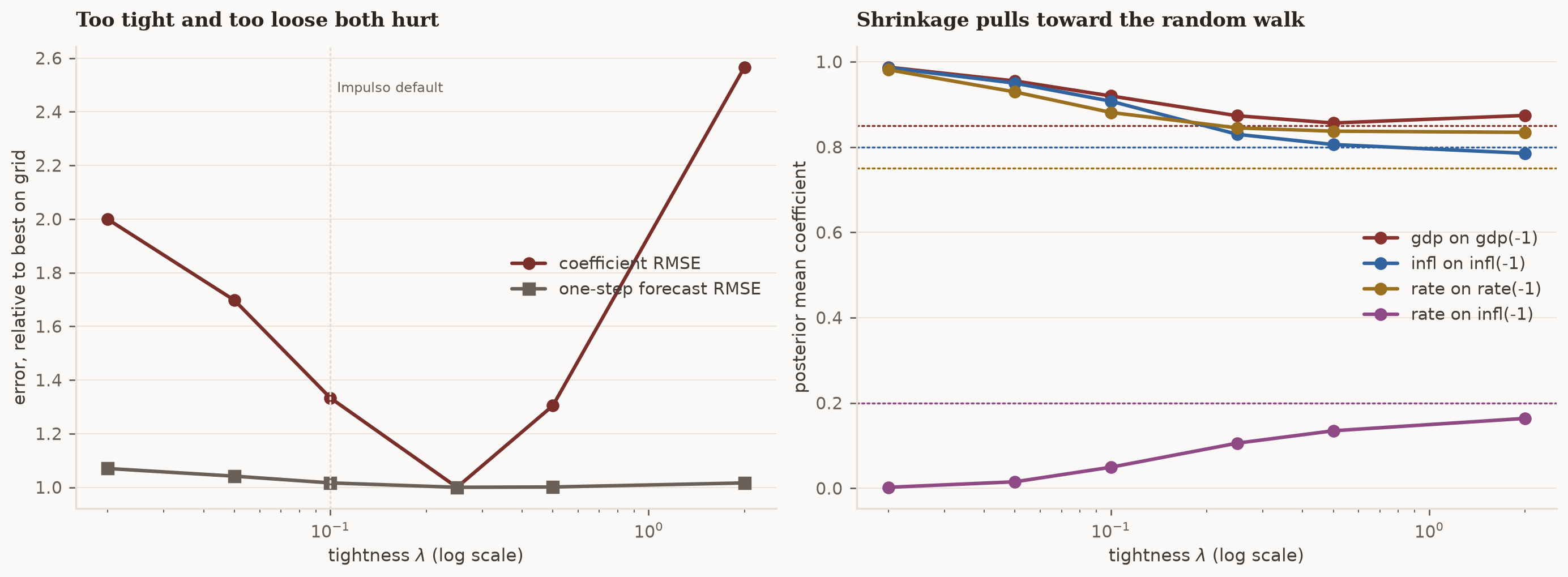
Fig. 6 Left: both error measures against tightness, each normalised by its own minimum so the two curves share an axis. Right: posterior means of the four largest true coefficients as tightness varies, with the true values as dotted lines. Loose priors overshoot the truth; very tight priors pin every coefficient to the random walk.

Both error curves are U-shaped, and that is the whole story in one picture. Move left and the prior overwhelms the data: at \(\lambda = 0.02\) every own-lag coefficient is pinned near 0.98 and every cross-lag coefficient near zero, whatever the sample says, so the model is biased. Move right and the prior stops doing anything: the estimates chase noise across 39 coefficients fitted on 100 observations, so the model is high-variance. Both ends are clearly worse than the middle.

On this grid the minimum sits at \(\lambda = 0.25\) rather than at the 0.1 default — but look at how flat the bottom of the curve is. Anything from 0.1 to 0.5 lands within two percent of the best forecast score available, whereas \(\lambda = 0.02\) costs seven percent, and both extremes roughly double the coefficient error. The lesson is not that 0.25 is the right number. It is that the decision worth making is an order of magnitude, and that the flat region is wide enough that a sensible default will not embarrass you.

Two honest caveats. The right panel shows shrinkage working against the truth for rate on infl(-1): its prior mean is 0 but its true value is 0.2, so every step toward a tighter prior biases it down. That is the deal you are taking — you accept bias on the handful of coefficients that are real to buy variance reduction on the many that are not. And the forecast curve is much flatter than the coefficient curve — the loose end barely hurts it at all — because one-step-ahead forecasts are dominated by the own first lag, the one coefficient the prior is least wrong about. The 27 badly estimated lag-2-to-4 coefficients hardly move a one-step forecast, which is why the coefficient panel is the sharper diagnostic. Shrinkage pays far more at longer horizons and in structural work, where those distant lags actually get used.

Choosing the settings

Situation	Suggested starting point
Small system (2–4 variables), long sample	tightness=0.2, cross_shrinkage=0.5 — you can afford to let the data speak
Standard macro VAR (5–8 variables)	The defaults: tightness=0.1, decay="harmonic", cross_shrinkage=0.5
Large system (10+ variables)	tightness=0.05 or lower — Giannone et al. [2015] show optimal tightness falls as \(n\) grows
Many lags on monthly or weekly data	decay="geometric" to kill distant lags, or decay="harmonic" if you expect seasonality
Forecasting benchmark	cross_shrinkage=0.0 — reduces the VAR to independent AR(\(p\)) models

Rather than trusting a table, fit two or three tightness values and compare. The prior predictive check above costs nothing and rules out the obviously bad end of the range; the held-out comparison settles the rest.

MinnesotaPrior does not rescale by variable

The classical Litterman formula multiplies the cross-variable standard deviation by \(\sigma_i / \sigma_j\), the ratio of residual scales, so that a coefficient linking a variable measured in basis points to one measured in log points is shrunk sensibly. Eq. 5 has no such term — build_priors only sees n_vars and n_lags, never your data. Put your variables on comparable scales before fitting, by standardising them or by expressing everything in percent. If you would rather the estimator handle scaling for you, NIWPrior computes per-variable AR(1) residual standard deviations internally; see The Conjugate VAR.

What the prior does not cover

MinnesotaPrior governs the lag coefficients only. Intercepts get a fixed \(\mathcal{N}(0, 1)\) prior, and the residual covariance \(\Sigma\) is handled by the volatility process (Constant by default, StochasticVolatility optionally). Standardising your data also keeps that \(\mathcal{N}(0, 1)\) intercept prior reasonable.

Where to go next

• Fit one end to end — the Quickstart walks through a full model with the default Minnesota prior.

• Let the data choose \(\lambda\) — The Conjugate VAR uses NIWPrior, whose conjugate structure gives a closed-form marginal likelihood, so the tightness can be selected rather than assumed (Giannone et al. [2015]).

• Write your own — Writing a Custom Prior shows the ten-line protocol any prior implements, which is how you would build the zero-mean or scale-aware variants mentioned above.

We currently have some availability for consulting on how Bayesian modelling, vector autoregressions, and impulso can be integrated into your team's macroeconomic and financial forecasting work. If this sounds relevant, book an introductory call. These calls are for consulting inquiries only. For technical usage questions and free community support, please use GitHub Discussions and the documentation.

References

The works cited above are collected on the project bibliography page.