Oil supply news with an external instrument

An OPEC announcement can move the oil price today even when it does not change production today. On 14 December 2006, for example, OPEC announced a cut of 500,000 barrels per day that would take effect the following February. Correspondingly, the oil price rose by about 2% on the announcement day as the market was reacting to news about future supply.

Känzig [2021] uses this timing to ask what happens after expectations of future oil supply deteriorate. The distinction from an unexpected loss of current production is important: Kilian [2009] shows that oil-price movements with different origins have different macroeconomic consequences. A shortage today forces users to draw down inventories. News of a shortage tomorrow instead gives them a reason to build inventories whilst oil is still available, which is why inventories carry identifying information in structural models of the oil market.

This tutorial reproduces Känzig’s six-variable oil-market VAR and then demonstrates how inference may be done in a Bayesian manner with Impulso. Identification is done through external instrument, or proxy [Stock and Watson, 2012, Mertens and Ravn, 2013], that we just described around changes in oil futures prices around OPEC announcements.

The aim is deliberately narrow. The proxy identifies the shock associated with news about future oil supply; it does not turn every oil-price movement into an oil supply shock, nor does it identify all the other shocks in the system.

How the announcement surprise identifies one shock

A VAR first removes the movements that can be predicted from past data. What remains is a vector of residuals, \(u_t\). These residuals are still mixtures: an unexpectedly high oil price in a given month could reflect supply news, demand news, geopolitical events, or several shocks at once. A structural VAR writes that mixture as

\[ u_t = P \varepsilon_t . \]

Here \(\varepsilon_t\) collects the unobserved economic shocks, whilst each column of \(P\) records how one of those shocks moves the six observed variables on impact.

Let \(z_t\) denote the futures-price change around an OPEC announcement. It can isolate the oil supply news shock, \(\varepsilon_{1t}\), under two assumptions [Mertens and Ravn, 2013, Stock and Watson, 2018]:

• Relevance: the announcement surprise moves with oil supply news, so \(\mathbb{E}[z_t \varepsilon_{1t}] = \phi \neq 0\).

• Exogeneity: it does not move systematically with the other structural shocks, so \(\mathbb{E}[z_t \varepsilon_{jt}] = 0\) for \(j \neq 1\).

Combining these two assumptions with the structural equation \(u_t = P \varepsilon_t\) gives the moment condition at the heart of the method:

\[ \mathbb{E}[z_t u_t] = P\, \mathbb{E}[z_t \varepsilon_t] = \phi\, p_1 . \]

This single equation is what makes the proxy approach work. The object we are after, \(p_1\), cannot be estimated directly, because the structural shocks \(\varepsilon_t\) are never observed; without further information, many different impact matrices \(P\) are equally consistent with the same fitted VAR. The moment condition resolves this by tying \(p_1\) to a quantity the data can deliver. When we multiply the residuals by the proxy and take expectations, exogeneity removes the contribution of all shocks other than oil supply news, whilst relevance guarantees that the surviving term is non-zero. The sample covariance between the proxy and the six VAR residuals is something we can compute directly once the VAR has been estimated and, therefore, points in the same direction as \(p_1\), the vector of impact effects we want. A series of announcement-day price changes, observed entirely outside the VAR, has told us which direction in residual space corresponds to oil supply news.

The one thing the covariance cannot reveal is the length of that vector, because the constant of proportionality \(\phi\) is unknown. The scale of the shock is therefore a modelling choice rather than an inferrable parameter. Following Känzig, we normalise the shock so that it raises the real oil price by 10% on impact, which makes every panel in the figures below readable as “the response to news that raises the oil price by 10%”. With the impact vector pinned down, the fitted VAR traces the responses of all six variables over subsequent months.

It is of note how little has been assumed here. The argument identifies only \(p_1\): it imposes no causal ordering among the six variables, as a recursive (Cholesky) identification would, and it places no sign or shape restrictions on any response. That restraint is what gives the results their evidential value. When inventories rise on impact and production falls only with a delay, the model has discovered the timing that distinguishes news from a current shortage, rather than being instructed to produce it.

import arviz as az
import matplotlib.pyplot as plt
import numpy as np
import pandas as pd
from qc_core import plotting

from impulso import VAR, VARData
from impulso.identification import ProxySVAR
from impulso.samplers import NUTSSampler

plotting.use_ledger_style()

Data: OPEC announcements and monthly macro variables

Känzig builds the proxy from 119 OPEC announcements between 1983 and 2017. For each announcement, the change in West Texas Intermediate (WTI) futures settlement prices from the last trading day before the announcement to the announcement day is recorded. Futures prices are used as OPEC production decisions usually take effect with a delay. The event-window design follows the high-frequency identification literature, which measures monetary policy surprises from federal funds futures around Federal Open Market Committee announcements [Kuttner, 2001, Gertler and Karadi, 2015]. If the futures risk premium does not change within the one-day window, the price change measures a revision in the expected future oil price.

The one-day window is a compromise. It gives markets time to interpret an OPEC statement, whose precise release time is often unavailable and whose contents may leak before publication. But a full day also leaves room for unrelated news to move oil prices. The proxy is therefore not automatically valid because it is measured at high frequency and its interpretation still rests on the exogeneity assumption above. Känzig studies this concern with control days, an alternative heteroskedasticity-based estimator, and several other checks; however, this tutorial focusses exclusively on the baseline external-instrument specification.

The files come from Känzig’s public replication repository (dkaenzig/replicationOilSupplyNews) and serve two different purposes:

• VAR data (monthly, 1974M01-2017M12): the real oil price, world oil production, world oil inventories, world industrial production, U.S. industrial production, and the U.S. consumer price index (CPI). The series enter as \(100 \times \log(\cdot)\), and the oil price is deflated by U.S. CPI.

• Proxy (indexed 1975M01-2017M12): the first principal component of announcement-day changes in WTI futures prices at maturities from 1 to 12 months. The underlying futures data begin in 1983. Surprises from multiple announcements in the same month are added together; a month without an announcement is recorded as zero, not as missing.

data_df = pd.read_csv("data/kaenzig_data.csv", index_col=0, parse_dates=True)
instrument = pd.read_csv("data/kaenzig_instrument.csv", index_col=0, parse_dates=True)[
    "oil_surprise"
]

var_names_paper = [
    "Real oil price",
    "World oil production",
    "World oil inventories",
    "World industrial production",
    "U.S. industrial production",
    "U.S. CPI",
]
data = VARData(
    endog=data_df.values, endog_names=list(data_df.columns), index=data_df.index
)

fig, ax = plt.subplots(figsize=(10, 3))
ax.plot(instrument.index, instrument.values, lw=0.8)
ax.set_ylabel("Oil price expectation revision [%]")
plotting.serif_title("Oil futures surprises around OPEC announcements", ax)

Text(0.0, 1.0, 'Oil futures surprises around OPEC announcements')

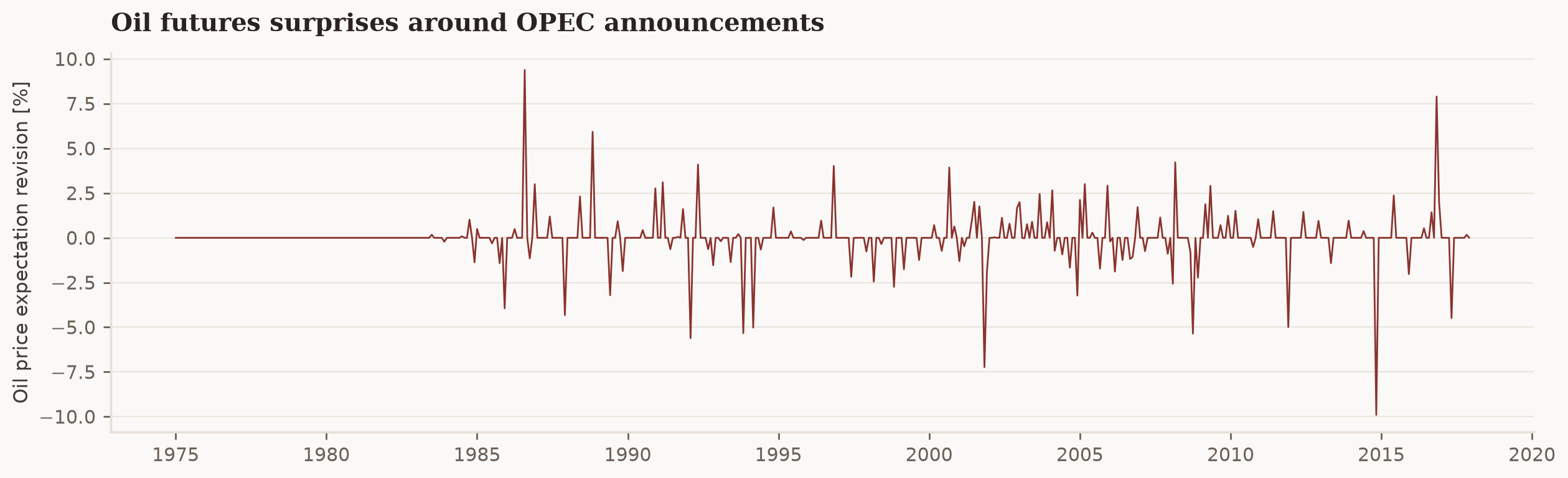
The series is sparse with long stretches of zeros punctuated by isolated spikes. This is because OPEC does not announce a new production decision every month, and a month without an announcement contributes a zero rather than a missing value. When the proxy is positive, futures prices rose around that month’s announcement, which Känzig reads as the market receiving adverse news about future supply: traders marked up the expected oil price because they expected less oil to be available. Negative values imply the inverse i.e., announcements that led the market to expect more future supply than it had previously priced in.

It is tempting to treat this series as a direct measurement of the oil supply news shock, but that would ask more of it than it can deliver. The announcement windows miss any supply news that arrives between OPEC meetings e.g., a pipeline outage or a conflict in a producing region, and each one-day window inevitably absorbs some unrelated price movement as measurement noise. The estimator therefore assigns the proxy a more modest role. Rather than entering the model as the shock, it indicates which combination of the VAR residuals co-moves with OPEC news, and the VAR itself supplies the shock series and its propagation.

First recover the published benchmark

Before changing the estimator, we reproduce the paper’s benchmark in NumPy. _kaenzig_frequentist.py follows the same sequence: estimate a 12-lag VAR in levels by ordinary least squares, use the announcement surprise as an instrument for the oil-price residual, and construct confidence bands with a moving-block bootstrap. Matching this result gives the Bayesian comparison a known reference point.

from _kaenzig_frequentist import first_stage_f, proxy_var_kaenzig, var_ols

nsim = 50 if ci else 1000
freq = proxy_var_kaenzig(
    data_df.values,
    instrument.values,
    p=12,
    horizon=50,
    shock_size=10.0,
    nsim=nsim,
    seed=0,
)

_, U_ols = var_ols(data_df.values, 12)
print(
    f"First stage: F = {first_stage_f(instrument.values, U_ols[:, 0]):.2f}, "
    f"robust F = {first_stage_f(instrument.values, U_ols[:, 0], robust=True):.2f}"
)

First stage: F = 22.67, robust F = 10.55

We are able to reproduce the first-stage F-statistic of 22.67 for the composite proxy and a heteroskedasticity-robust value of 10.55 that Känzig reports. The proxy explains 4.22% of the monthly oil-price residual, which is enough signal to be useful, but not so much that instrument strength can be ignored. The conventional \(F>10\) rule is only a screening device, and the robust result sits just above it. An F-statistic also says nothing about exogeneity: a strong instrument can still be invalid.

What changes in the Bayesian version

The economic design and the dynamic specification stay fixed. We still use the same six variables, 12 monthly lags, a constant, and the same proxy. What changes is how the reduced-form VAR and its uncertainty are estimated.

Step	Känzig’s benchmark	Impulso version
VAR coefficients	Ordinary least squares	Bayesian posterior with a Minnesota prior
Identification	One impact vector from the external instrument	The external-instrument impact vector, estimated for every posterior draw
Uncertainty	Moving-block bootstrap	Posterior credible intervals, conditional on the observed proxy series

Of these differences, it is the prior that carries economic meaning. The Minnesota prior centres each equation on a univariate random walk, with the first own lag at one and every remaining lag coefficient at zero, and lets the data pull the posterior away only where the evidence warrants. Such shrinkage is consequential in a system of this size as, with six variables and 12 lags, each equation contains 72 lag coefficients. The low-rank mass-matrix setting supplied to the sampler below is different in kind. It helps NUTS negotiate the strong posterior correlations among these coefficients and embodies no additional economic assumption.

By contrast, the proxy’s role is unchanged from the frequentist setup whereby it serves identification, not estimation. Although the impact vector is computed separately for each posterior draw, the instrument never enters the likelihood, so the reduced-form posterior is informed by the VAR data alone. Fully Bayesian proxy SVARs, in which the instrument is modelled jointly with the VAR so that it also informs the reduced-form posterior, are developed by Caldara and Herbst [2019] and Arias et al. [2021].

if ci:
    sampler = NUTSSampler(
        draws=50,
        tune=500,
        chains=1,
        cores=1,
        target_accept=0.9,
        random_seed=42,
        nuts_sampler_kwargs={"low_rank_modified_mass_matrix": True},
    )
else:
    sampler = NUTSSampler(
        draws=1000,
        tune=1500,
        chains=2,
        cores=1,
        target_accept=0.9,
        random_seed=42,
        nuts_sampler_kwargs={"low_rank_modified_mass_matrix": True},
    )

fitted = VAR(lags=12, prior="minnesota").fit(data, sampler=sampler)

summ = az.summary(fitted.idata, var_names=["B"], kind="diagnostics")
print(
    f"B coefficients: min ESS = {summ['ess_bulk'].min():.0f}, "
    f"median ESS = {summ['ess_bulk'].median():.0f}, "
    f"max r_hat = {summ['r_hat'].max():.3f}"
)
print(f"divergences: {int(fitted.idata.sample_stats['diverging'].sum())}")

B coefficients: min ESS = 1555, median ESS = 2334, max r_hat = 1.010
divergences: 0

The full run reports no divergences, a large minimum bulk effective sample size, and a maximum \(\hat R\) of 1.01. Those diagnostics give us a reassuring set of posterior draws for the comparison. For more detail on what each of these diagnostics catches, and on repairing a fit that fails them, see the Model Checks and Validation tutorial, which diagnoses and resolves slow mixing in a levels VAR using the same low-rank mass-matrix setting employed above.

Once the VAR has been fitted, identification is one additional step. For each posterior draw, ProxySVAR reconstructs the monthly residuals and calculates how they co-move with the announcement surprise. Dates are matched through the two DatetimeIndex objects. Months missing from the proxy are dropped, whilst zero-valued months stay in the calculation, because a zero is an observation in its own right: it records that no OPEC announcement occurred.

We orient the shock so that adverse supply news raises the oil price. Setting scale=10.0 then applies Känzig’s normalisation: the real oil price rises by 10% on impact.

scheme = ProxySVAR(
    instrument=instrument,
    policy_variable="real_oil_price",
    shock_name="oil_supply_news",
    scale=10.0,
)
ivar = fitted.set_identification_strategy(scheme)
irf = ivar.impulse_response(horizon=50)

The structural shock matrix stores a summary of the first-stage diagnostics; however, we can also inspect the full distribution. The instrument is fixed across draws, but the reconstructed oil-price residual changes with the VAR coefficients and so each draw, therefore, implies a different first-stage F-statistic:

sm = ivar.shock_matrix()
{k: round(v, 2) for k, v in sm.attrs.items()}

{'proxy_first_stage_f_median': 23.22,
 'proxy_first_stage_f_q05': 21.71,
 'proxy_first_stage_f_q95': 24.72,
 'proxy_impact_cache_hit': 0.0}

f_draws = scheme.first_stage(fitted.idata.posterior, data, n_lags=12).ravel()

fig, ax = plt.subplots(figsize=(6, 3.2))
ax.hist(f_draws, bins=40, color=plotting.COLORS.oxblood, alpha=0.75)
ax.axvline(
    10,
    color=plotting.COLORS.ink,
    ls="--",
    lw=1,
    label="F = 10 rule of thumb",
)
ax.axvline(
    np.median(f_draws),
    color="C1",
    lw=1.5,
    label=f"posterior median = {np.median(f_draws):.1f}",
)
ax.set_xlabel("First-stage F")
plotting.serif_title("Posterior of instrument relevance", ax)
plotting.legend_below(ax, per_row=2)

<matplotlib.legend.Legend at 0x7f9deebfb8d0>

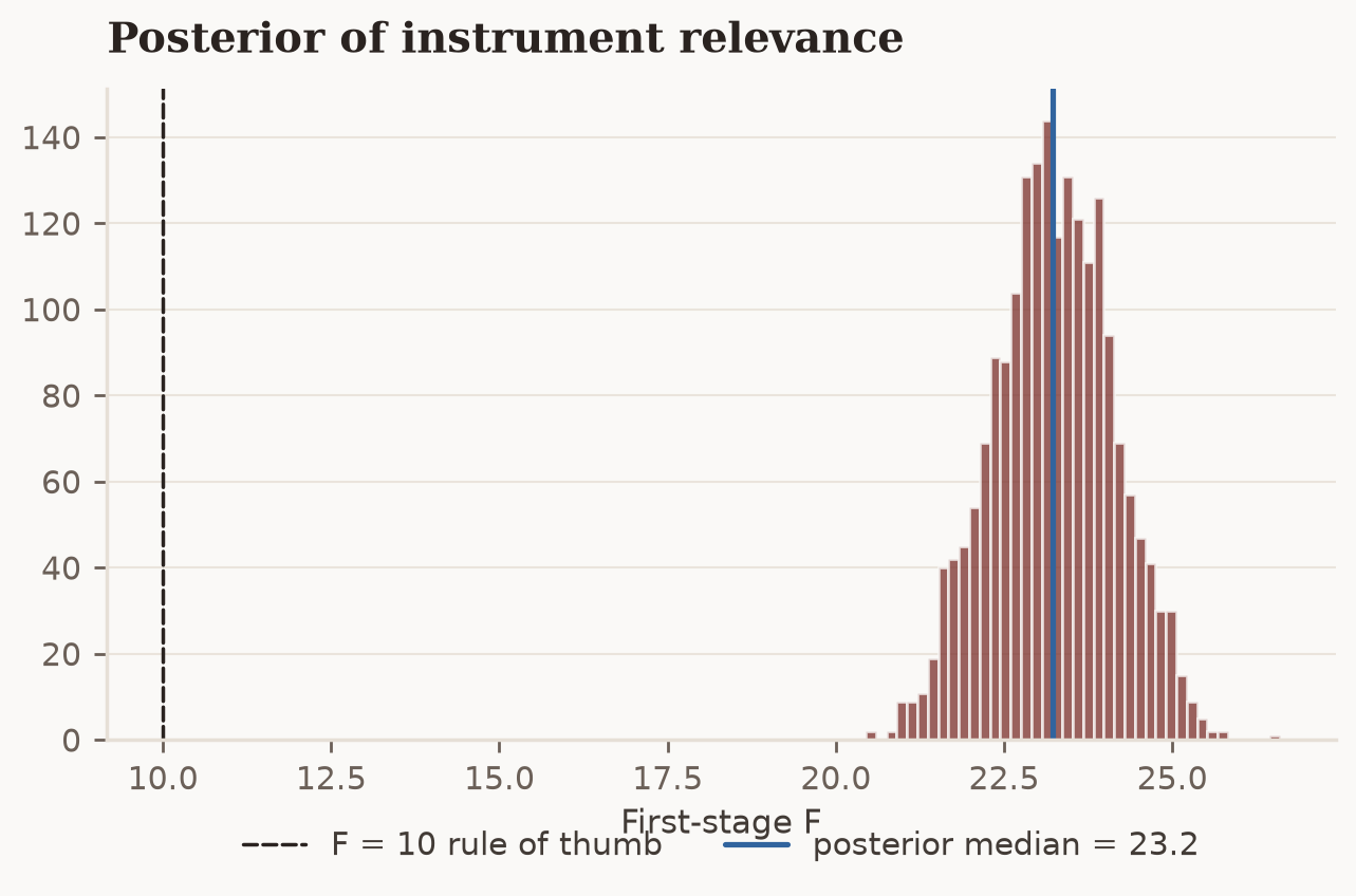
All of the posterior mass lies above the \(F=10\) rule of thumb, which is reassuring about relevance but cannot settle the exclusion question. Further, the histogram is not a bootstrap of the announcement series, as the proxy is held fixed throughout, and the spread comes entirely from uncertainty about the fitted VAR. The distribution matters because identification is repeated for every draw. Each draw’s impact vector is estimated from its own first stage, and the 10% normalisation divides by that draw’s oil-price impact, so draws with a weak first stage push erratic responses into the credible bands. Because little of the mass sits below ten here, the bands in the next section can be read as economic uncertainty rather than as a symptom of weak identification.

What follows adverse oil supply news?

The figure overlays two analyses of the same six-variable system. The solid ledger accent shows the Impulso posterior median with 68% and 90% credible intervals. The dashed comparison shows a local reproduction of Känzig’s OLS point estimate and moving-block-bootstrap confidence bands, the resampling scheme that Jentsch and Lunsford [2019] recommend for proxy SVARs. The paper uses 10,000 bootstrap replications but in this notebook we use 1,000 to keep the compilation manageable. These intervals have different interpretations, so their widths should not be read as a contest between methods. The useful comparison is whether the estimated paths tell a similar economic story.

irf_draws = irf.idata.posterior_predictive["irf"].sel(shock="oil_supply_news")
med = irf_draws.median(dim=("chain", "draw")).values
q = {
    p: irf_draws.quantile(p, dim=("chain", "draw")).values
    for p in (0.05, 0.16, 0.84, 0.95)
}

horizon = np.arange(51)
fig, axes = plt.subplots(2, 3, figsize=(11, 7), sharex=True)
for j, (ax, name) in enumerate(zip(axes.ravel(), var_names_paper)):
    ax.fill_between(
        horizon,
        q[0.05][:, j],
        q[0.95][:, j],
        alpha=0.18,
        color="C0",
        label="Impulso 90%",
    )
    ax.fill_between(
        horizon,
        q[0.16][:, j],
        q[0.84][:, j],
        alpha=0.35,
        color="C0",
        label="Impulso 68%",
    )
    ax.plot(horizon, med[:, j], color="C0", lw=1.8, label="Impulso median")
    ax.plot(horizon, freq.irf[:, j], color="C1", lw=1.5, ls="--", label="Känzig point")
    for lo, hi in (freq.bands68, freq.bands90):
        ax.plot(horizon, lo[:, j], color="C1", lw=0.8, ls=":")
        ax.plot(horizon, hi[:, j], color="C1", lw=0.8, ls=":")
    ax.axhline(0, color=plotting.COLORS.hairline, lw=0.6)
    plotting.serif_title(name, ax, fontsize=11)
    ax.set_xlim(0, 50)
    if j >= 3:
        ax.set_xlabel("Months")
    if j % 3 == 0:
        ax.set_ylabel("%")
axes[0, 0].legend()
fig.suptitle(
    "Response to an oil supply news shock raising the real oil price by 10%",
    y=1.0,
    fontfamily=plotting.SERIF_STACK,
    fontweight=600,
)

Text(0.5, 1.0, 'Response to an oil supply news shock raising the real oil price by 10%')

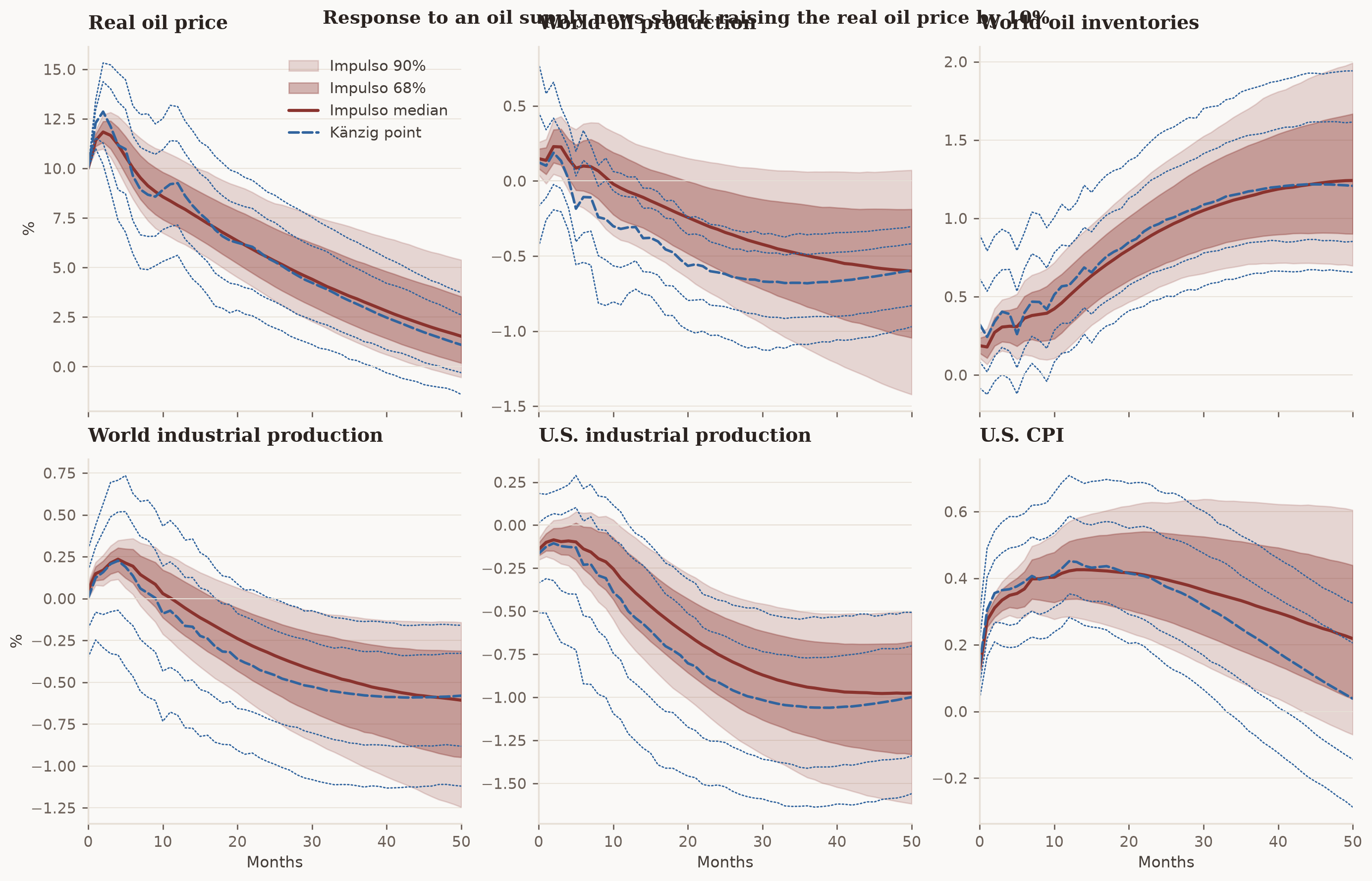
The first three panels depict the central economic result that oil prices rises by construction. However, oil production changes little on impact and declines only later, whilst inventories begin to rise immediately. That is the timing predicted by news of a future shortfall whereby firms store oil before supply tightens. An unexpected shortfall today would instead force production down and inventories to be used. Because the model imposes none of these signs, the pattern is evidence in favour of the interpretation rather than a restatement of the identifying assumptions.

The news also propagates beyond the oil market. World industrial production is nearly unchanged during the first year and then falls. U.S. industrial production declines sooner and more sharply, whilst the U.S. price level rises. In Känzig’s estimates, a shock that raises the oil price by 10% eventually lowers world oil production by about 0.7%, raises inventories by 1.2%, lowers world and U.S. industrial production by 0.6% and 1%, and raises U.S. CPI by about 0.4%. The Impulso medians closely reproduce those magnitudes and dynamics.

The two sets of bands also differ in width, and the difference changes with the horizon. Over the first year or two the Impulso credible intervals are markedly tighter than the bootstrap bands, but they widen steadily thereafter, and by month 50 the two are of comparable width, with the Impulso bands, if anything, the wider for world oil production. Both patterns follow from how each method handles parameter uncertainty. Each bootstrap replicate re-estimates the unregularised OLS system and the first-stage regression on resampled data, so noise in the 72 lag coefficients of every equation, and in the instrument’s co-movement with the residuals, enters the comparison bands from the first month. Impulso instead conditions on the observed proxy and shrinks the lag coefficients towards a random walk, so its short-horizon responses are tightly determined, and in the oil-price panel the impact is fixed at exactly 10% in every draw by the normalisation.

The clearest difference appears in U.S. CPI after about 30 months, where Impulso’s posterior median decays more slowly than Känzig’s point estimate, though the published path remains inside the 90% credible interval. Random-walk shrinkage of the persistent CPI series is a plausible explanation, but establishing it would require a prior-sensitivity exercise, and Giannone et al. [2015] show how the tightness of such priors can itself be inferred from the data. The comparison here also covers only the paper’s baseline external-instrument design. Känzig’s checks for event-window noise and alternative specifications remain important evidence for the economic interpretation.

Extension: allow the shock scale to change over time

Känzig’s benchmark uses one residual covariance matrix, \(\Sigma\), for the full sample. The next analysis is an extension rather than part of the replication, as Impulso can replace that constant matrix with a sequence, \(\Sigma_t\), thus allowing the model to represent calm and volatile periods differently [Cogley and Sargent, 2005, Primiceri, 2005]. The proxy continues to determine which residual direction represents oil supply news, whilst the time-varying covariance determines how large a one-standard-deviation shock is in each month. For the volatility model itself, from the univariate case through to the multivariate volatility="sv" form used below, see the Stochastic Volatility tutorial, which also documents the at= interface for extracting per-period results.

To keep the notebook practical to render, we fit this stochastic-volatility model to four variables: the real oil price, world oil production, U.S. industrial production, and U.S. CPI. The same API accepts the six-variable system, but that model contains more than 3,000 latent volatility states. Because the system is smaller, the results below demonstrate the extension and should not be treated as a direct robustness check of the six-variable benchmark.

core = ["real_oil_price", "world_oil_production", "us_ip", "us_cpi"]
data_sv = VARData(endog=data_df[core].values, endog_names=core, index=data_df.index)

if ci:
    sv_sampler = NUTSSampler(
        draws=50,
        tune=500,
        chains=1,
        cores=1,
        target_accept=0.9,
        random_seed=42,
        nuts_sampler_kwargs={"low_rank_modified_mass_matrix": True},
    )
else:
    # Sized to the docs CI cell budget: nutpie runs chains in parallel, so the
    # cell's wall time tracks one chain's tune+draws. Heavier settings (e.g.
    # tune=2000, draws=1000, chains=4) push this cell past the 1800 s
    # nb_execution_timeout on CI runners; the interrupted sampler then returns
    # a NaN-padded posterior (see NUTSSampler's incomplete-draw guard).
    sv_sampler = NUTSSampler(
        draws=500,
        tune=1000,
        chains=2,
        cores=1,
        target_accept=0.9,
        random_seed=42,
        nuts_sampler_kwargs={"low_rank_modified_mass_matrix": True},
    )

fitted_sv = VAR(lags=12, volatility="sv").fit(data_sv, sampler=sv_sampler)

summ_sv = az.summary(fitted_sv.idata, var_names=["B"], kind="diagnostics")
print(
    f"B coefficients: min ESS = {summ_sv['ess_bulk'].min():.0f}, "
    f"max r_hat = {summ_sv['r_hat'].max():.3f}, "
    f"divergences: {int(fitted_sv.idata.sample_stats['diverging'].sum())}"
)

B coefficients: min ESS = 356, max r_hat = 1.010, divergences: 1

The diagnostics of the stochastic-volatility fit are less clean than the baseline; however, they are adequate for demonstrating how the interfaces compose, but not for a final empirical analysis. A substantive application should run longer and resolve the divergences before interpreting the time-varying scale.

With time-varying volatility, shock_matrix(at="all") returns an impact matrix for every month rather than a single one. The entry worth plotting is the one that links the oil supply news shock to the real oil price. For each month \(t\), it answers a concrete question: “had a typical oil supply news shock arrived that month, one standard deviation in size under \(\Sigma_t\), by how many percent would the real oil price have moved on impact?”. The direction of the shock in residual space is pinned down by the proxy and never changes. What changes is the amount of residual variation along that direction, which \(\Sigma_t\) lets expand in turbulent periods and contract in calm ones. Keeping the 10% normalisation would erase exactly this variation by forcing the answer to be 10 in every month, so we set scale=None and let the model report the shock’s natural size. In the figure below, the line is the posterior median of that month-by-month impact and the band is a 68% credible interval.

scheme_sd = ProxySVAR(
    instrument=instrument,
    policy_variable="real_oil_price",
    shock_name="oil_supply_news",
)
ivar_sd = fitted_sv.set_identification_strategy(scheme_sd)
sd_path = ivar_sd.shock_matrix(at="all").sel(
    response="real_oil_price", shock="oil_supply_news"
)
sd_med = sd_path.median(dim=("chain", "draw"))
sd_lo = sd_path.quantile(0.16, dim=("chain", "draw"))
sd_hi = sd_path.quantile(0.84, dim=("chain", "draw"))

fig, ax = plt.subplots(figsize=(10, 3.5))
t = sd_path.coords["time"].values
ax.fill_between(t, sd_lo, sd_hi, alpha=0.3, color="C0")
ax.plot(t, sd_med, color="C0", lw=1.2)
ax.set_ylabel("% oil price impact")
plotting.serif_title("One-standard-deviation oil supply news shock, period by period", ax)

Text(0.0, 1.0, 'One-standard-deviation oil supply news shock, period by period')

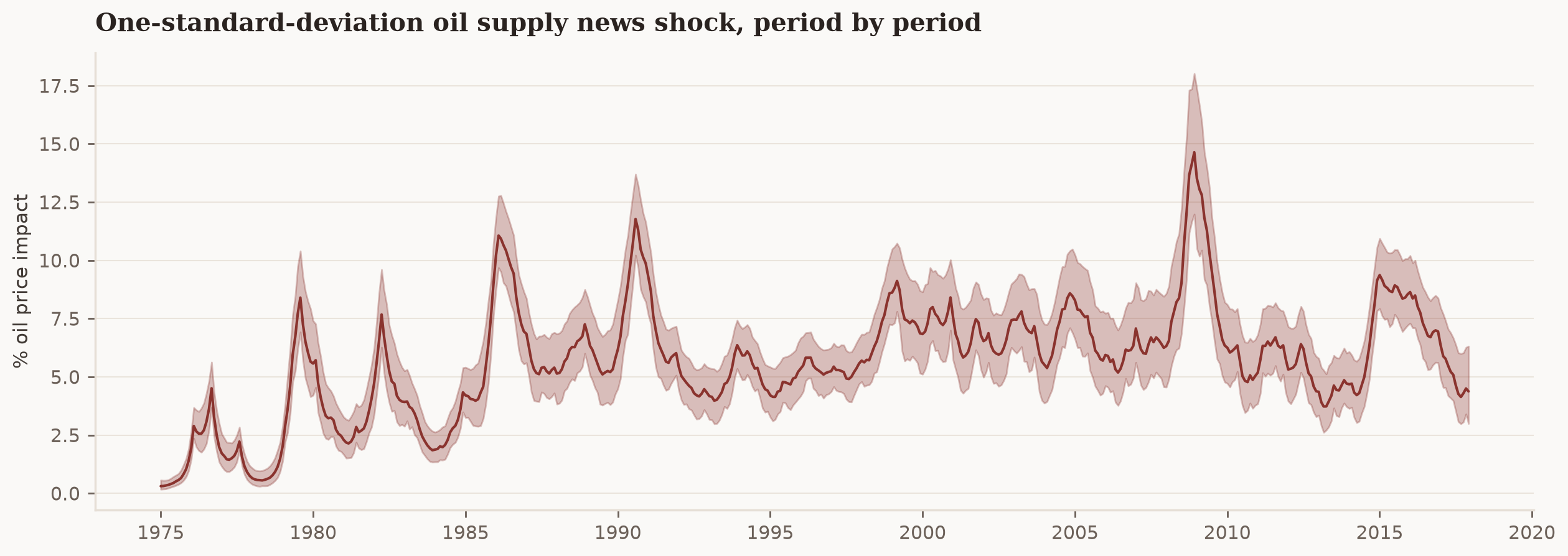
The scale moves several-fold over the sample, and its peaks sit on familiar episodes of oil-market turbulence, including the 1979-80 oil crisis, the 1986 price collapse, the Gulf War, and the 2008-09 financial crisis. At the 1986 and 1990-91 peaks a typical shock moved the oil price by around 11% on impact, whereas through the calm mid-1990s the same one-standard-deviation event was worth closer to 5%. The 2008-09 peak, the largest in the sample, is also a helpful guide to what the path measures. That episode is usually attributed to collapsing demand, so the plot is tracking the changing scale of the residuals rather than dating occasions of oil supply news, and it is not a historical decomposition. A constant-\(\Sigma\) model would compress this whole path into one average scale.

The boundary of the identification

The proxy identifies one column of the impact matrix. Some downstream calculations need a square, invertible matrix, so Impulso fills in the other columns with an orthogonal completion and labels them unidentified_*. These columns are computational placeholders, in the sense that rotating them would change neither the identified oil supply news shock nor the reduced-form covariance.

The result methods preserve that distinction:

• fevd() asks how much forecast-error variance each shock explains. It reports the share attributable to oil supply news but returns NaN for each unidentified_* share, because those individual shares change under an arbitrary rotation. FEVD also requires one-standard-deviation shocks, so use scale=None rather than the 10% normalisation.

• historical_decomposition() attributes the deviation of the observed path from its deterministic baseline to shocks over time. It combines the unidentified columns into unidentified_remainder: their separate paths are arbitrary, but their sum is the part not attributed to oil supply news.

• ProxySVAR emits a warning when the posterior-median first-stage F-statistic is below 10. The warning flags weak relevance; it cannot diagnose a violation of exogeneity.

Reproducing this notebook

The data CSVs ship with the documentation. To rebuild them from the original files, clone dkaenzig/replicationOilSupplyNews and follow mainAnalysisOilSupplyNews.m: transform the variables to \(100 \times \log(\cdot)\), deflate the oil price by CPI, and use column 15 for the principal-component futures surprise. A full render fits two MCMC models and takes about fifteen minutes on a laptop.

References

The works cited above are collected on the project bibliography page.