Probabilistic Forecasts

Conventional VARs produce point forecasts. A Bayesian VAR produces a full posterior predictive distribution over future paths. This means every forecast comes with calibrated uncertainty — wide bands when the model is unsure, narrow when the data are informative.

That uncertainty has two sources: the model’s coefficients are only estimated, and the system is hit by a fresh random shock every period. forecast() includes both by default. The section below shows why leaving the shocks out — as much VAR tooling implicitly does — understates uncertainty, badly so at short horizons.

import numpy as np
import pandas as pd

from impulso import VAR, VARData
from impulso.samplers import NUTSSampler

Setup

We repeat the data-generating process from the quickstart tutorial. The DGP is a VAR(1) with three macro variables — GDP growth, inflation, and an interest rate. If you’ve already worked through that notebook, the setup code below will be familiar.

rng = np.random.default_rng(42)
T = 200
n_vars = 3

A_true = np.array([
    [0.6, 0.0, -0.1],
    [0.2, 0.5, 0.0],
    [0.0, 0.15, 0.4],
])

y = np.zeros((T, n_vars))
for t in range(1, T):
    y[t] = A_true @ y[t - 1] + rng.standard_normal(n_vars) * 0.1

index = pd.date_range("2000-01-01", periods=T, freq="QS")
data = VARData(endog=y, endog_names=["gdp_growth", "inflation", "rate"], index=index)

sampler = NUTSSampler(draws=500, tune=500, chains=2, cores=1, random_seed=42)
fitted = VAR(lags=1, prior="minnesota").fit(data, sampler=sampler)
fitted

FittedVAR(n_lags=1, data=VARData(endog_names=['gdp_growth', 'inflation', 'rate'], exog_names=None), var_names=['gdp_growth', 'inflation', 'rate'], volatility=Constant(name='constant', is_time_varying=False, sigma_sd_beta=2.5, tril_offdiag_sigma=0.5))

Point forecasts

Call .forecast(steps=8) to produce an 8-step-ahead forecast. The result is a ForecastResult object that holds the full posterior predictive draws. The .median() method extracts the central tendency — the posterior median at each horizon.

fcast = fitted.forecast(steps=8)
fcast.median()

	gdp_growth	inflation	rate
0	-0.009484	0.074313	-0.056796
1	-0.006551	0.045508	-0.031101
2	-0.003114	0.024710	-0.011212
3	-0.002359	0.004380	-0.004237
4	-0.006467	-0.003285	-0.004171
5	-0.001610	-0.013397	-0.012227
6	-0.004527	-0.017316	-0.012945
7	-0.003210	-0.017350	-0.006051

Each row is a forecast horizon (1 through 8 quarters ahead). The values converge toward the unconditional mean of the process as the horizon increases — a hallmark of stationary VARs.

Credible intervals

The .hdi() method computes the highest density interval at a given probability level. An 89% HDI means 89% of the posterior forecast mass falls within these bounds. We use 89% rather than 95% following the ArviZ convention — it avoids the false precision of round numbers.

hdi = fcast.hdi(prob=0.89)

print("Lower bounds:")
print(hdi.lower)
print("\nUpper bounds:")
print(hdi.upper)

Lower bounds:
   gdp_growth  inflation      rate
0   -0.169762  -0.080550 -0.198768
1   -0.202939  -0.164066 -0.215112
2   -0.216438  -0.165644 -0.204400
3   -0.200668  -0.197332 -0.195431
4   -0.220686  -0.201912 -0.180370
5   -0.227766  -0.223935 -0.184484
6   -0.249458  -0.222047 -0.200863
7   -0.223059  -0.227592 -0.206168

Upper bounds:
   gdp_growth  inflation      rate
0    0.139566   0.242779  0.090906
1    0.182586   0.224295  0.137757
2    0.196226   0.245744  0.169363
3    0.218451   0.208549  0.185046
4    0.212144   0.220640  0.196537
5    0.208693   0.211567  0.190625
6    0.185708   0.218958  0.176971
7    0.208036   0.204679  0.159339

The intervals widen at longer horizons. This is expected: two forces compound over time — the random shocks hitting the system accumulate, and parameter uncertainty propagates forward as each forecast step feeds into the next.

Visualise the forecast

The .plot() method produces a fan chart showing the median forecast with shaded credible bands for each variable.

fig = fcast.plot()

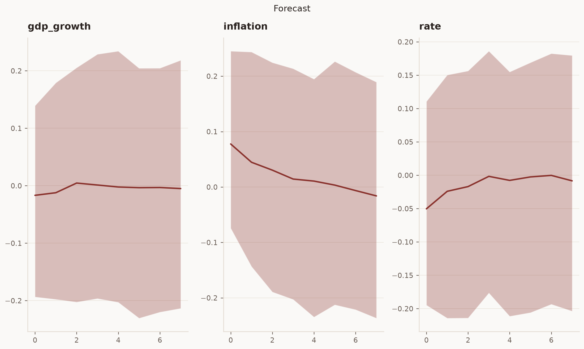
The fan chart shows the posterior median (line) and 89% HDI (shaded region) for each variable. The bands widen at longer horizons, reflecting compounding uncertainty. GDP growth and the interest rate show the widest bands, consistent with their stronger cross-variable dependencies in the DGP.

What the bands include

The forecast above is a genuine posterior predictive distribution: it composes parameter uncertainty (the coefficients are estimated, not known) with shock uncertainty (each future period draws a fresh innovation). This is the default — include_shock_uncertainty=True.

Setting include_shock_uncertainty=False switches the shocks off and propagates only the posterior over conditional-mean paths. The result is a distribution over what the model expects to happen, not over what will happen. It is the right object for scenario mechanics, but it is not a predictive distribution — and reporting it as one is a common way to understate forecast uncertainty. Pass seed in density mode to make the drawn shocks reproducible.

mean_fcast = fitted.forecast(steps=8, include_shock_uncertainty=False)
density_fcast = fitted.forecast(steps=8, include_shock_uncertainty=True, seed=42)

mean_hdi = mean_fcast.hdi(prob=0.89)
density_hdi = density_fcast.hdi(prob=0.89)

Plotting both 89% bands on the same axes shows the gap. The narrow inner band is parameter uncertainty alone; the wider band is the full predictive.

import matplotlib.pyplot as plt

horizons = range(1, 9)
fig, axes = plt.subplots(1, n_vars, figsize=(12, 4), squeeze=False)

for i, name in enumerate(data.endog_names):
    ax = axes[0][i]
    med = density_fcast.median()[name].values
    ax.fill_between(
        horizons, density_hdi.lower[name], density_hdi.upper[name],
        alpha=0.25, color="C0", label="full predictive",
    )
    ax.fill_between(
        horizons, mean_hdi.lower[name], mean_hdi.upper[name],
        alpha=0.5, color="C1", label="parameter only",
    )
    ax.plot(horizons, med, color="black", lw=1)
    ax.set_title(name)
    ax.set_xlabel("horizon")

axes[0][0].legend(loc="upper left", fontsize=8)
fig.tight_layout()

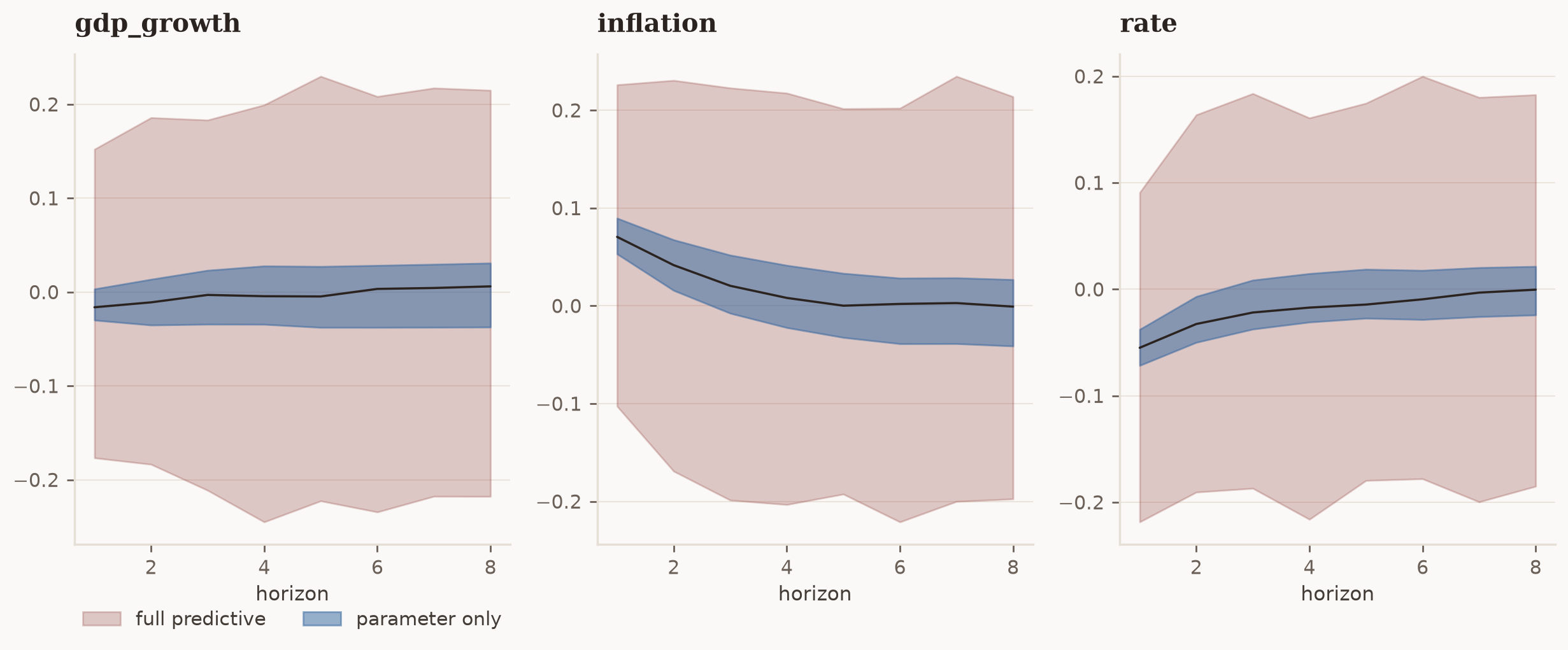
The understatement is worst at the shortest horizons. At h=1, parameter uncertainty is small — the data pin the coefficients down — so a mean-only band is almost invisible, yet the true one-step forecast still carries the full shock variance. The ratio of band widths makes this concrete:

width_mean = mean_hdi.upper - mean_hdi.lower
width_density = density_hdi.upper - density_hdi.lower

ratio = (width_density / width_mean).round(1)
ratio.index = range(1, 9)
ratio.index.name = "horizon"
ratio

	gdp_growth	inflation	rate
horizon
1	9.9	9.0	9.1
2	7.6	7.7	8.2
3	6.9	7.1	8.1
4	7.1	6.6	8.3
5	7.0	6.0	7.7
6	6.7	6.3	8.2
7	6.5	6.5	8.2
8	6.3	6.1	8.1

Each entry is how many times wider the honest band is than the parameter-only band. The multiple is largest at h=1 and shrinks as parameter uncertainty grows into the total — the opposite of the intuition that near-term forecasts are the certain ones.

Tidy export

For downstream analysis or dashboarding, .to_dataframe() returns the median forecast in a tidy DataFrame format.

fcast.to_dataframe()

	gdp_growth	inflation	rate
step
0	-0.009484	0.074313	-0.056796
1	-0.006551	0.045508	-0.031101
2	-0.003114	0.024710	-0.011212
3	-0.002359	0.004380	-0.004237
4	-0.006467	-0.003285	-0.004171
5	-0.001610	-0.013397	-0.012227
6	-0.004527	-0.017316	-0.012945
7	-0.003210	-0.017350	-0.006051

Summary

Bayesian VAR forecasts provide more than point predictions. The full posterior predictive distribution lets you quantify and communicate forecast uncertainty honestly. For structural questions — what happens to inflation when the central bank raises rates? — see the Structural Analysis tutorial.

We currently have some availability for consulting on how Bayesian modelling, vector autoregressions, and impulso can be integrated into your team's macroeconomic and financial forecasting work. If this sounds relevant, book an introductory call. These calls are for consulting inquiries only. For technical usage questions and free community support, please use GitHub Discussions and the documentation.