Counterfactuals, conditional forecasts, and structural scenarios

“What if” analysis in the style of Antolín-Díaz, Petrella & Rubio-Ramírez (2021)

Every policy debate is a “what if”. What would food prices have done without the energy shock? What does the forecast look like if the central bank holds rates at 2% for a year? And if it does, which shocks have to do the work — and how believable are they?

Impulso answers these three questions with one family of tools, built on a single stacked-shock engine (Antolín-Díaz et al. [2021]):

Question	Method	Where it lives
What would history have looked like without shock \(j\)?	counterfactual()	IdentifiedVAR
What is the forecast if variable \(i\) follows path \(x\)?	conditional_forecast()	FittedVAR
Same path, but only named shocks may absorb it — and how plausible is that?	structural_scenario()	IdentifiedVAR

The conditional forecast (Waggoner and Zha [1999]) lets every structural shock adjust, and its answer is provably invariant to the identification scheme — which is why it lives on the reduced-form object and needs no identification at all. The structural scenario restricts who adjusts, which is where identification starts to matter. And every scenario ships with a plausibility statistic in the tradition of Leeper and Zha [2003]’s “modest policy interventions”: a measure of how hard the model has to be pushed to deliver your scenario.

The Lucas critique still applies

All three tools hold the estimated reduced-form dynamics fixed while editing or constraining shocks. That is a fixed-path intervention, not a change of policy rule: if agents’ behaviour would change under the scenario (as Leeper and Zha [2003] formalise), the model’s answer degrades — and degrades faster the less “modest” the intervention. The plausibility statistic is the guard rail: treat scenarios it flags as incredible with corresponding scepticism.

import matplotlib.pyplot as plt
import numpy as np
import pandas as pd
from qc_core import plotting

from impulso import VAR, VARData, ShockPath, VariablePath
from impulso.identification import Cholesky
from impulso.samplers import NUTSSampler

plotting.use_ledger_style()

Data and model

We reuse the three-variable U.S. monetary system from the monetary policy tutorial: log industrial production (output), the log consumer price index (CPI, prices), and the federal funds rate (rate), monthly from 1965 to December 2007 — the eve of the zero-lower-bound era, which makes the forecast-side scenarios below historically pointed.

Antolín-Díaz et al. [2021] run their scenario analysis on a richer quarterly system with sign, narrative, and long-run identification. Impulso’s v1 machinery covers the scenario engine in full; here we identify the monetary shock with a standard recursive (Cholesky) ordering instead, so the numbers below are methodological companions to that paper, not a replication of its tables. The calibrated plausibility scale is theirs, and reads the same way.

df = pd.read_csv("data/monetary_policy.csv", index_col="date", parse_dates=True)
df = df.loc[:"2007-12"]

if ci:
    sampler = NUTSSampler(
        draws=50,
        tune=500,
        chains=1,
        cores=1,
        target_accept=0.9,
        random_seed=123,
        nuts_sampler_kwargs={"low_rank_modified_mass_matrix": True},
    )
else:
    sampler = NUTSSampler(
        draws=1500,
        tune=1500,
        chains=4,
        cores=4,
        random_seed=123,
        target_accept=0.9,
        nuts_sampler="nutpie",
    )

data = VARData.from_df(df, endog=["output", "prices", "rate"])
fitted = VAR(lags=12, prior="minnesota").fit(data, sampler=sampler)
identified = fitted.set_identification_strategy(Cholesky(ordering=["output", "prices", "rate"]))

Under this ordering the third structural shock — the one that moves the funds rate on impact without contemporaneously moving output or prices — is the monetary policy shock. It is labelled rate in every result below.

1. Historical counterfactual: the Volcker disinflation without the shocks

Between October 1979 and mid-1982 the Federal Reserve under Paul Volcker pushed the funds rate to unprecedented levels. Through the lens of the vector autoregression (VAR), that period contains a sequence of large monetary policy shocks: movements in the rate not explained by the systematic response to output and prices.

counterfactual() asks: what if those shocks had simply not happened? It backs out the realised structural shocks for every posterior draw, switches the monetary shock off over the window (values=0.0), and re-propagates the system from the actual initial conditions. Realised shocks are edited, never re-drawn, so the band below reflects parameter and identification uncertainty only.

cf = identified.counterfactual(
    shocks=[ShockPath(shock="rate", values=0.0, start="1979-10-01", end="1982-08-01")],
    start="1978-01-01",
    end="1986-12-01",
)
fig = cf.plot()

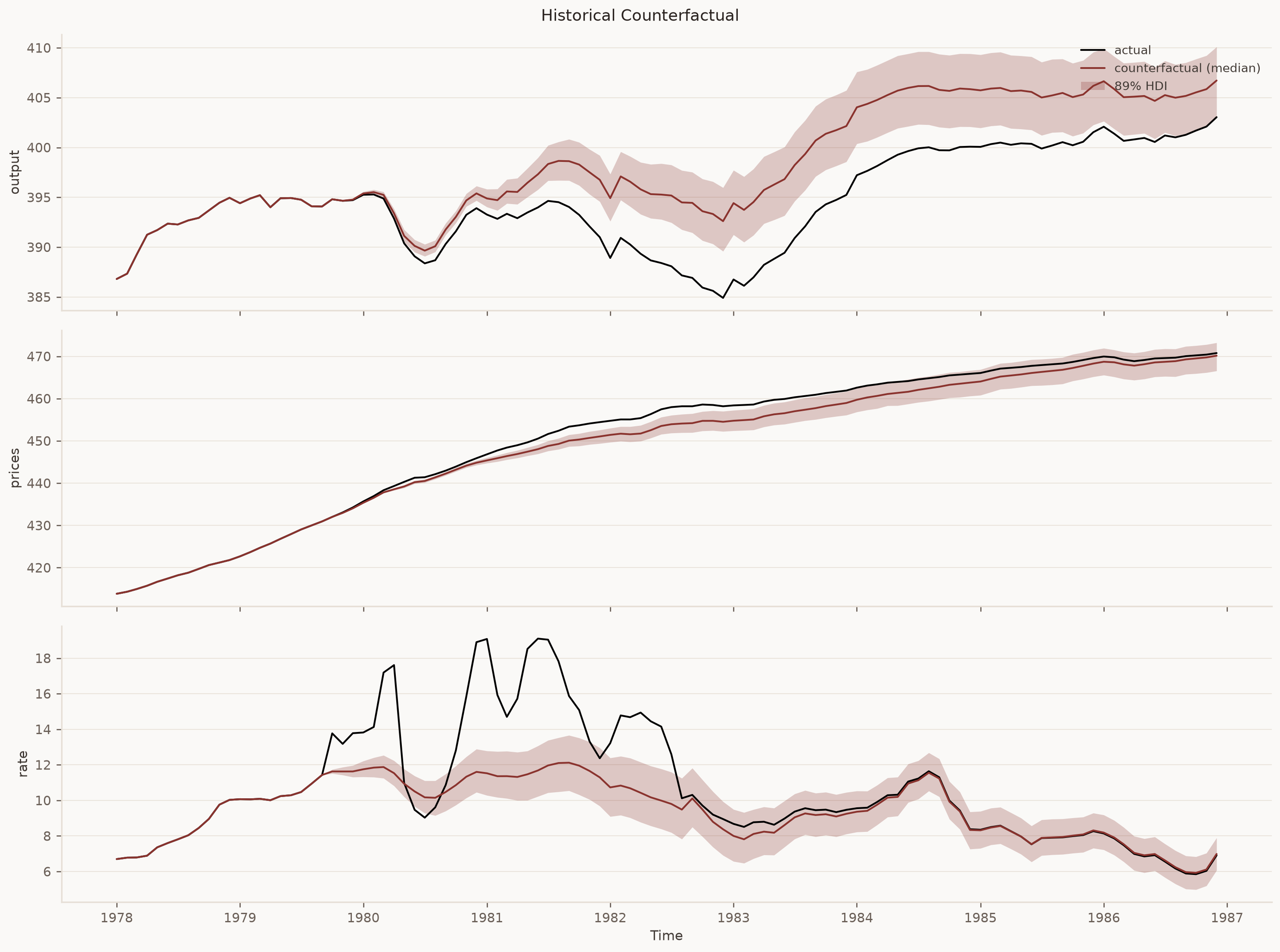
Fig. 19 Actual paths vs the counterfactual in which the monetary policy shock is switched off from October 1979 to August 1982. The shaded band is the counterfactual’s 89% highest density interval (HDI).

The difference() accessor gives the median effect of the edit — here, the cumulative contribution of the Volcker-era monetary shocks to each series. Two properties of this object are worth knowing. First, for a shock zeroed over the full sample, actual - counterfactual equals that shock’s historical-decomposition contribution exactly, draw by draw — the two features answer the same question with the same numbers. Second, a windowed edit is a different object: the difference is zero before the window, and persists after it (the economy does not snap back to the actual path when the edit window closes), because the counterfactual carries its own lag dynamics forward.

cf.difference().loc["1980-01-01":"1983-01-01"].round(2).head(8)

	output	prices	rate
time
1980-01-01	-0.13	0.31	2.07
1980-02-01	-0.24	0.41	2.29
1980-03-01	-0.37	0.51	5.31
1980-04-01	-0.52	0.77	6.08
1980-05-01	-0.75	1.09	0.04
1980-06-01	-1.05	1.05	-1.04
1980-07-01	-1.28	0.89	-1.14
1980-08-01	-1.41	0.76	-0.54

2. Conditional forecast: pinning the 2008 easing path

Our sample ends in December 2007. Over the following year the Federal Reserve cut the funds-rate target from 4.25% to nearly zero. We now stand at the end of 2007 and ask: given a rate path like the one that unfolded, what does the model expect for output and prices?

conditional_forecast() pins future values of chosen variables and lets all structural shocks adjust (Waggoner and Zha [1999]). Pins hold pathwise on every draw; unpinned entries keep their full predictive uncertainty. NaN entries in a pinned path mean “unconstrained at that step”.

# The approximate 2008 federal-funds target path (policy meetings, rounded).
easing_path = np.array([3.0, 3.0, 2.25, 2.0, 2.0, 2.0, 2.0, 2.0, 2.0, 1.0, 1.0, 0.25])

cf_2008 = fitted.conditional_forecast(
    steps=12,
    conditions=[VariablePath(variable="rate", values=easing_path)],
    seed=123,
)
fig = cf_2008.plot()

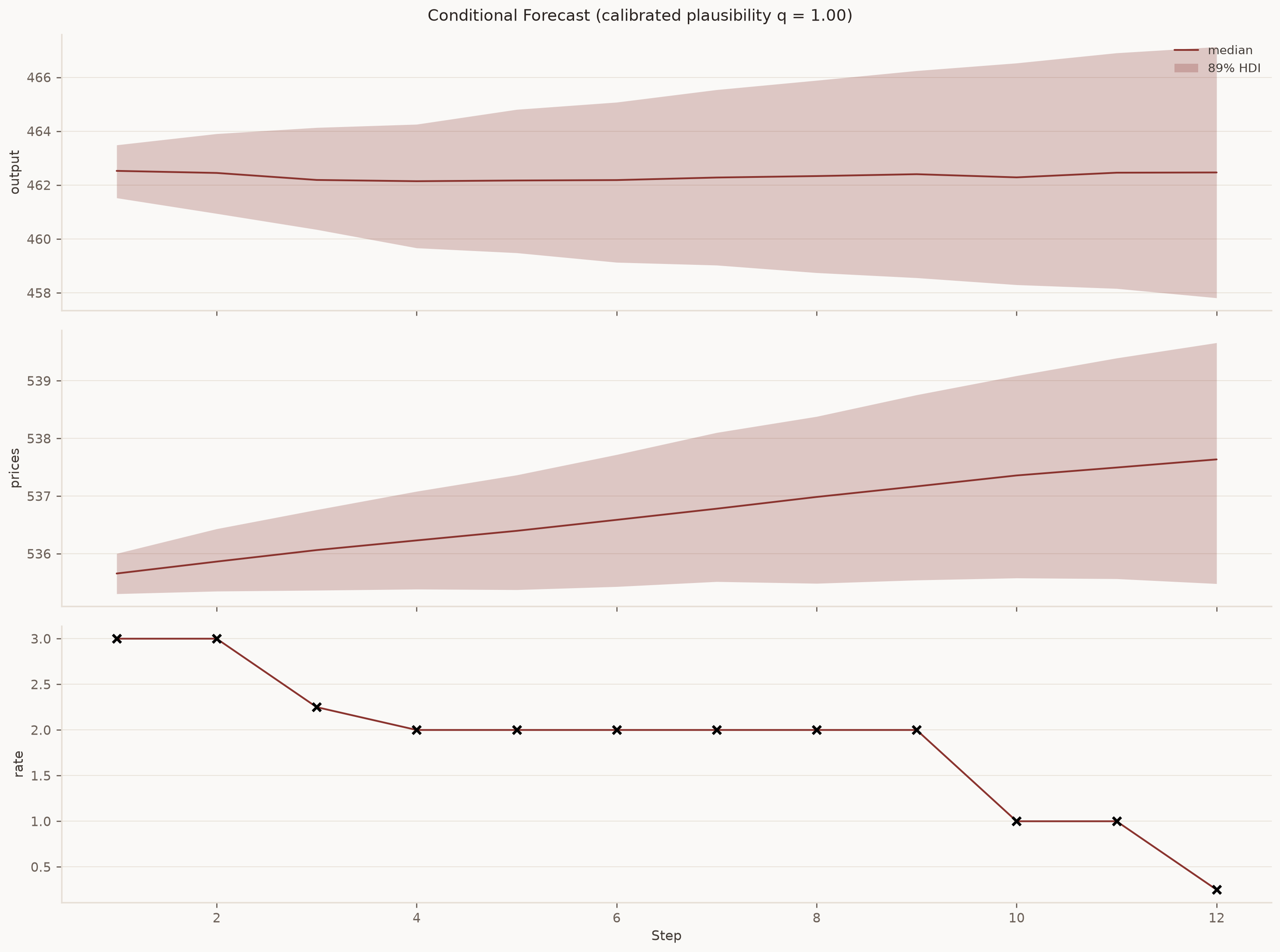
Fig. 20 Conditional forecast for 2008 with the funds rate pinned to the approximate easing path actually followed. Crosses mark the pinned values.

3. Structural scenario: who does the work, and is it believable?

The conditional forecast is agnostic about why the rate follows the path — demand, supply, and policy shocks all conspire to deliver it. A structural scenario (Antolín-Díaz et al. [2021]) names the shocks allowed to absorb the conditions. Setting adjusting=["rate"] loads the entire easing onto monetary policy shocks while demand and supply shocks keep their unconditional distributions — the scenario reads “the Fed chooses this path”.

Every solve-path result carries two plausibility diagnostics, reported per posterior draw:

• q — the squared Mahalanobis distance of the pinned values from their unconditional distribution (\(\chi^2_r\) reference when all shocks adjust): how many standard-deviations-worth of shocks the scenario demands.

• q_cal — the calibrated statistic of Antolín-Díaz et al. [2021] on \([0.5, 1]\) (via McCulloch [1989]): \(0.5\) means “indistinguishable from the unconditional forecast”, values near \(1\) mean “incredible”. Under hard pins the underlying divergence is infinite and q_cal sits at its ceiling of 1 by construction; the informative version uses path_uncertainty="unconditional", which restricts the forecast mean only and keeps honest bands — the mode behind that paper’s headline numbers.

scenario = identified.structural_scenario(
    steps=12,
    conditions=[VariablePath(variable="rate", values=easing_path)],
    adjusting=["rate"],
    path_uncertainty="unconditional",
    seed=123,
)
fig = scenario.plot()

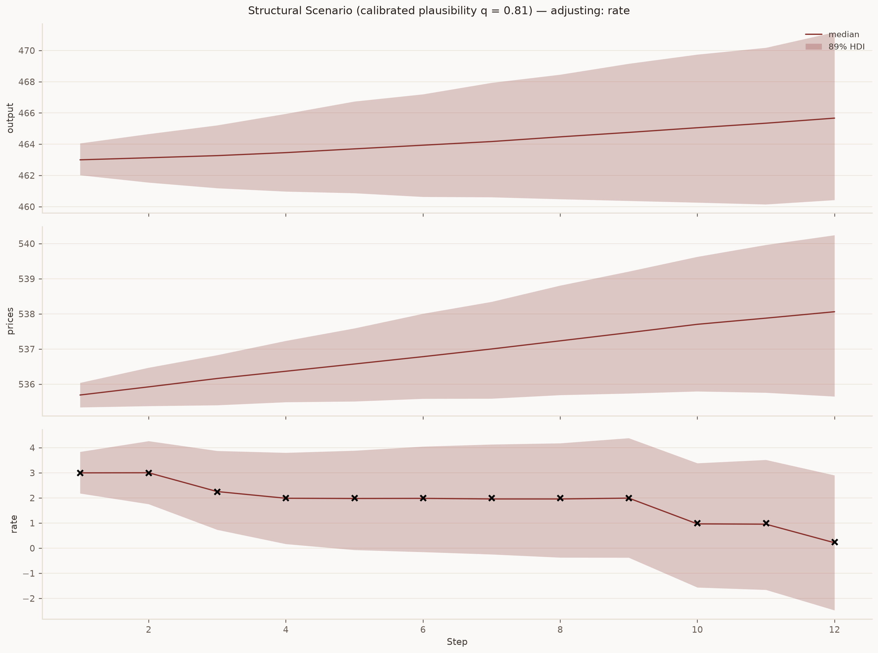
Fig. 21 Structural scenario: the same easing path, absorbed entirely by monetary policy shocks, with unconditional-width bands (path_uncertainty=’unconditional’).

How believable are competing 2008 policy paths as pure policy choices? We compare the easing that happened against an alternative “hold at 4.25%” path, in the mean-restricting mode:

hold_path = np.full(12, 4.25)
rows = {}
for name, path in {"2008 easing": easing_path, "hold at 4.25%": hold_path}.items():
    scn = identified.structural_scenario(
        steps=12,
        conditions=[VariablePath(variable="rate", values=path)],
        adjusting=["rate"],
        path_uncertainty="unconditional",
        seed=123,
    )
    summary = scn.plausibility()
    rows[name] = {
        "q (median)": round(summary["q_median"], 1),
        "calibrated q": round(summary["q_calibrated_median"], 2),
    }
pd.DataFrame(rows).T

	q (median)	calibrated q
2008 easing	17.5	0.81
hold at 4.25%	1.0	0.58

Read the calibrated column on the Antolín-Díaz–Petrella–Rubio-Ramírez scale. Their empirical anchors run from a posterior mode near \(0.5\) for a scenario they call quite realistic, through \(0.83\) for one they call “unlikely but not completely implausible”, to results near \(0.86\) that they say should be interpreted with caution; their hard-restriction variants peg the metric at its ceiling of \(1\), a large distortion of the shock distribution. (The paper reports posterior modes; the table above shows medians.) A scenario that demands a long sequence of same-signed monetary shocks — the model’s way of saying “this is not what my estimated policy rule would do” — earns a higher q than one the rule largely delivers on its own.

You can also prescribe future shock paths directly (shocks=[ShockPath(...)] on the forecast axis): the prescribed magnitude then enters the plausibility statistic as \(\lVert v_S \rVert^2\), so a prescribed three-standard-deviation shock registers as \(q \mathrel{+}= 9\) even though it is substituted outright.

Summary

1. counterfactual() edits realised structural shocks and re-propagates — the in-sample “what if”, dual to the historical decomposition.

2. conditional_forecast() pins future observable paths with all shocks free — identification-free by construction.

3. structural_scenario() names the adjusting shocks and/or prescribes shock paths — and its plausibility statistics tell you when to stop believing the answer.

The three methods share one engine and one vocabulary (ShockPath, VariablePath), and their overlaps are exact: a structural scenario with every shock adjusting is the conditional forecast (draw for draw under the recursive identification and matched seeds used here), and a full-sample zero-edit counterfactual is the historical decomposition, draw for draw.

Reproducing this notebook

Full-fidelity builds sample 4 chains × 1,500 draws with nutpie; CI smoke builds (IMPULSO_DOCS_CI=1) shrink to a single short chain, so smoke-mode bands are wider and attribution noisier. Given the posterior and a fixed seed, the plausibility statistics are exactly reproducible (with a proper adjusting set, q also varies with the free shocks’ draws), and because the two rate paths differ by many standard-deviations-worth of monetary shocks, the ordering of the scenario table should be insensitive to the sampling mode.

References

The works cited above are collected on the project bibliography page.